Week 11 - Simulation of Flow through a pipe in OpenFoam

Problem Statement:

Simulate flow through a pipe where the flow is laminar, incompressible, and transient.

Edit the blockMeshDict file in icoFoam solver using Matlab Code which will generate the computational mesh automatically for any wedge angle and grading schemes.

Plot velocity profile for the fully developed flow.

Post-process velocity and shear stress.

Introduction:

The flow through pipes is usually involved in heating, cooling, and fluid distribution network applications. The fluid is forced to flow through the pipe with the help of a pump which gives an initial velocity in this case is 0.17m/s. Mostly circular pipes are used for the transport of fluids because circular pipes can withstand larges pressure differences between inside and outside without undergoing significant distortion.

The fluid velocity inside the pipe changes from zero at the wall because of the no-slip condition to the maximum at the center. It is convenient to work with an average velocity which remains constant for the incompressible flow as the cross-sectional area of the pipe is constant. The average velocity changes at heating and cooling applications because of changes with temperature and density. But here the fluid properties are evaluated at some average temperature and treated as constants.

Laminar flow is characterized by smooth streamline and highly ordered motion of the fluid particles.

Turbulent flow is characterized by velocity fluctuations and disordered motion of the fluid particles.

Reynolds Number: It is the ratio of inertia force to viscous force.

When Reynolds number is low which indicates that there is a large viscous force present which suppresses the fluctuations and maintains the ordered motion of the fluid molecules in other words the flow is laminar.

When Reynolds number is high large inertia forces are present which causes disorderedness in the motion of the molecule in other words the flow is turbulent.

`R_e`< = 2300 Laminar flow

`R_e` >= 4000 Turblent Flow.

2300`<=` `R_e``<=` 4000 Transistion flow.

The flow region where the viscous shearing forces due to fluid viscosity is felt is called the velocity boundary layer also called the boundary layer. Due to this hypothetical layer divides the flow region into a boundary layer where the viscous effects are felt and changes in the velocity are significant and an irrotational flow region where the frictional effects are negligible and velocity is constant.

The thickness of the boundary layer increases in the direction of the fluid flow until the reaches the center of the pipe and velocity is fully developed at a distance from the inlet.

The distance from the inlet of the pipe to a point where the velocity is fully developed is called hydrodynamic entrance length.

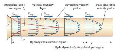
In the hydrodynamic entrance region, shear wall stress is highest at the inlet of the pipe and where the thickness of the boundary layer is minimum and shear stress decreases along the fluid flow direction to fully developed flow.

Entry length

The hydrodynamic entry length is taken to be the distance from the entrance region to the point where the shear stress is about 2 percent of the fully developed flow.

L/D = 0.005Re.

Velocity profile can be calculated as

`u = 2*V_(avg)*(1-(r)^2/(R)^2)`

where u is velocity profile in m/s.

`V_(avg)` is the average velocity in m/s.

r is the radial distance in m.

R is the radius of the pipe in m.

The maximum velocity is at the center of the pipe which can be obtained by substituting r=0 in the above formula

`V_(max) = 2* V_(avg)`

Hagen Poiseuille Equation:

Hagen Poiseuille equation evaluates the pressure drop in an incompressible and Newtonian fluid in a laminar flow that has a constant cross-sectional area and also the length of the pipe should be larger than its diameter.

Assumptions in this equation are that the fluid is an incompressible and Newtonian fluid whose length is larger than its diameter.

This equation calculates pressure drop due to viscosity in the fluid.

The equation to calculate the pressure drop is given by:

`triangleP = (128*mu*L*Q)/(pi*D^4)`

where Q is the volumetric flow rate in `m^3/s`

D is the diameter of the pipe in m.

L is the length of the pipe in m.

`mu` is the dynamic viscosity in `kg.m^-1.s^-1`

Pressure Drop

Pressure drop is calculated as it is related to the power requirement of the pump to maintain the flow inside the pipe.

Pressur drop can also be calculated using the below formula.

`(dp)/dx = (P_2-P_1)/L`

`triangleP = (8* mu*L*V_(avg))/R^2`

`mu` is a dynamic viscosity in `kg.m^-1.s-1`.

L is the length of the pressure drop region.

`V_(avg)` is the average velocity in m/s.

R is the radius of the pipe in m.

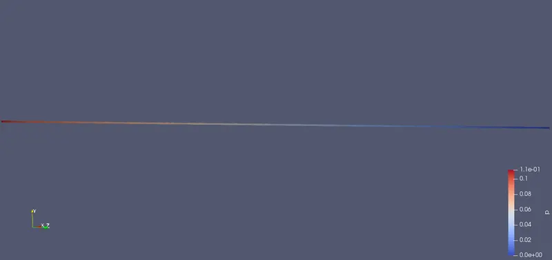
From the above formula, the pressure loss is proportional to viscosity which when its value is zero then there is no pressure drop. Therefore the pressure drop from P1 to P2 is entirely due to viscous for constant diameter and fixed length of the pipe.

Matlab Code to automate the computational mesh for any wedge angle.

% Code to automate the computational mesh for any wedge angle
close all 
clear all
clc

%Defining the wedge angle from which the vertices are calculated using
%trignometry fucntions.
theta = 5;
theta =  theta/2;
x = cosd(theta)*0.005;
y = sind(theta)*0.005;
%length of the pipe.
l = 2;

%Creating a blockMeshDict file 
f = fopen('blockMeshDict.txt','w');

%Below are the codes for blockMeshDict file.
fprintf (f ,'%s n' ,'/*--------------------------------*- C++ -*----------------------------------*');
fprintf (f,'%s n','  =========                 |');
fprintf (f,'%sn','        /  F ield         | OpenFOAM: The Open Source CFD Toolbox');
fprintf (f,'%sn','       /   O peration     | Website:  https://openfoam.org');
fprintf (f,'%sn','      /    A nd           | Version:  8');
fprintf (f,'%sn','     /     M anipulation  |');
fprintf (f,'%sn','*---------------------------------------------------------------------------*/');
fprintf (f,'%sn','FoamFile');
fprintf (f,'%sn','{');
fprintf (f,'%sn','');
fprintf (f,'%sn','    version     2.0;');
fprintf (f,'%sn','    format      ascii;');
fprintf (f,'%sn','    class       dictionary;');
fprintf (f,'%sn','    object      blockMeshDict;');
fprintf (f,'%sn','}');
fprintf (f,'%sn','// * * * * * * * * * * * * * * * * * * * * * * * * * * * * * * * * * * * * * //');
fprintf (f,'%sn','');
fprintf (f,'%sn','convertToMeters 1;');
fprintf (f,'%sn','');
fprintf (f,'%sn','vertices');
fprintf (f,'%sn','(');
fprintf (f,'%sn','    (0 0 0)');
fprintf (f,'%sn','    (0 0 0)');
fprintf (f,'%s %f %f %f %s n','    (',y,x,0,')'); %<-- giving the calculated values as vertices for defining the wedge
fprintf (f,'%s %f %f %f %s n','    (',-y,x,0,')');
fprintf (f,'%s %f %f %f %s n','    (',0,0,l,')');
fprintf (f,'%s %f %f %f %s n','    (',0,0,l,')');
fprintf (f,'%s %f %f %f %s n','    (',y,x,l,')');
fprintf (f,'%s %f %f %f %s n','    (',-y,x,l,')');
fprintf (f,'%sn',');');
fprintf (f,'%sn','');
fprintf (f,'%sn','blocks');
fprintf (f,'%sn','(');
fprintf (f,'%sn','    hex (0 1 2 3 4 5 6 7) (1 50 200) simpleGrading (1 0.1 1)');
fprintf (f,'%sn',');');
fprintf (f,'%sn','');
fprintf (f,'%sn','edges');
fprintf (f,'%sn','(');
fprintf (f,'%sn',');');
fprintf (f,'%sn','');
fprintf (f,'%sn','boundary');
fprintf (f,'%sn','(');
fprintf (f,'%sn','    inlet');
fprintf (f,'%sn','    {');
fprintf (f,'%sn','        type patch;');
fprintf (f,'%sn','        faces');
fprintf (f,'%sn','        (');
fprintf (f,'%sn','            (0 3 2 1)');
fprintf (f,'%sn','        );');
fprintf (f,'%sn','    }');
fprintf (f,'%sn','');
fprintf (f,'%sn','     outlet');
fprintf (f,'%sn','    {');
fprintf (f,'%sn','        type patch;');
fprintf (f,'%sn','        faces');
fprintf (f,'%sn','        (');
fprintf (f,'%sn','            (4 7 6 5)');
fprintf (f,'%sn','        );');
fprintf (f,'%sn','    }');
fprintf (f,'%sn','');
fprintf (f,'%sn','    fixedWalls');
fprintf (f,'%sn','    {');
fprintf (f,'%sn','        type wall;');
fprintf (f,'%sn','        faces');
fprintf (f,'%sn','        (');
fprintf (f,'%sn','            (3 2 6 7)');
fprintf (f,'%sn','        );');
fprintf (f,'%sn','    }');
fprintf (f,'%sn','    wedge1');
fprintf (f,'%sn','    {');
fprintf (f,'%sn','        type wedge;');
fprintf (f,'%sn','        faces');
fprintf (f,'%sn','        (');
fprintf (f,'%sn','            (0 3 7 4)');
fprintf (f,'%sn','        );');
fprintf (f,'%sn','    }');
fprintf (f,'%sn','     wedge2');
fprintf (f,'%sn','    {');
fprintf (f,'%sn','        type wedge;');
fprintf (f,'%sn','        faces');
fprintf (f,'%sn','        (');
fprintf (f,'%sn','            (1 5 6 2)');
fprintf (f,'%sn','        );');
fprintf (f,'%sn','    }');
fprintf (f,'%sn','    line1');
fprintf (f,'%sn','    {');
fprintf (f,'%sn','    	type empty;');
fprintf (f,'%sn','    	faces');
fprintf (f,'%sn','    	(');
fprintf (f,'%sn','    		(0 1 5 4)');
fprintf (f,'%sn','        );');
fprintf (f,'%sn','    }');
fprintf (f,'%sn','');
fprintf (f,'%sn',');');
fprintf (f,'%sn','');
fprintf (f,'%sn','mergePatchPairs');
fprintf (f,'%sn','(');
fprintf (f,'%sn',');');
fprintf (f,'%sn','');
fprintf (f,'%sn','// ************************************************************************* //');
fprintf (f,'%sn','');

Explanation of the Matlab code:

In the above code, the desired wedge angle is defined for the theta variable which is used to calculate the vertices for the wedge angle, and also the length of the pipe is defined in variable l.

BlockMeshDict.txt file is created to which codes are written which are similar to the original blockMeshDict which includes the vertices for the model, defining of the model satisfying right-hand thumb rule and also defining the type of boundary conditions along with the faces of the wedge.

Created BlockMeshDict file using the above Matlab code for wedge angle 5 degrees.

/*--------------------------------*- C++ -*----------------------------------* 
  =========                 | 
        /  F ield         | OpenFOAM: The Open Source CFD Toolbox
       /   O peration     | Website:  https://openfoam.org
      /    A nd           | Version:  8
     /     M anipulation  |
*---------------------------------------------------------------------------*/
FoamFile
{

    version     2.0;
    format      ascii;
    class       dictionary;
    object      blockMeshDict;
}
// * * * * * * * * * * * * * * * * * * * * * * * * * * * * * * * * * * * * * //

convertToMeters 1;

vertices
(
    (0 0 0)
    (0 0 0)
    ( 0.000218 0.004995 0.000000 ) 
    ( -0.000218 0.004995 0.000000 ) 
    ( 0.000000 0.000000 2.000000 ) 
    ( 0.000000 0.000000 2.000000 ) 
    ( 0.000218 0.004995 2.000000 ) 
    ( -0.000218 0.004995 2.000000 ) 
);

blocks
(
    hex (0 1 2 3 4 5 6 7) (1 50 200) simpleGrading (1 0.1 1)
);

edges
(
);

boundary
(
    inlet
    {
        type patch;
        faces
        (
            (0 3 2 1)
        );
    }

     outlet
    {
        type patch;
        faces
        (
            (4 7 6 5)
        );
    }

    fixedWalls
    {
        type wall;
        faces
        (
            (3 2 6 7)
        );
    }
    wedge1
    {
        type wedge;
        faces
        (
            (0 3 7 4)
        );
    }
     wedge2
    {
        type wedge;
        faces
        (
            (1 5 6 2)
        );
    }
    line1
    {
    	type empty;
    	faces
    	(
    		(0 1 5 4)
        );
    }

);

mergePatchPairs
(
);

// ************************************************************************* //

Explanation:

In the above code, the first seven lines contain the header information and the code information is in a foam file which is enclosed in '{}'.

After the file information, the dimensions are converted into meters by multiplying the scaling factor by 1.

Then vertices for wedge block are defined using the Right-hand thumb rule in which the z-axis is normal to the surface.

Blocks are defined after the definition of vertices for the blocks where the hex is defining the shape of the block which is hexahedra. The order of the vertices in defining the block should be done carefully because this line also specifies a local axis for the vertices to which the number of cells is defined along with grading. Here simple grading is cell expansion. In the parenthesis, we specify the ratio which is the width of the end cell along one edge of a block to the width of the start cell along that edge.

Since there are no curved edges in the geometry it is left empty i.e., no points are specified within the parenthesis. The reason for not including arc for the top surface of the wedge is due to the small wedge angle which does not affect the end results of the simulation.

Boundary Conditions:

For the inlet and outlet, the type of boundary conditions specified are:

type: patch type on which particular boundary conditions are applied and faces: mean a list of block faces that make up the patch. The type of Boundary conditions chosen is inlet velocity and outlet pressure.

FixedWalls is of wall type since particular physical properties are defined at these walls, in this case, is the dynamic viscosity in `kg.m^-1s^-1`

Wedge 1 and Wedge2 walls are of type wedge because there is no solution required since the flow considered is 2D flow. Type is empty is defined for the wedge because walls defined for type empty should be parallel to each other which is not satisfied in this case hence type wedge is chosen.

Initial Conditions for Pressure:

/*--------------------------------*- C++ -*----------------------------------*
  =========                 |
        /  F ield         | OpenFOAM: The Open Source CFD Toolbox
       /   O peration     | Website:  https://openfoam.org
      /    A nd           | Version:  8
     /     M anipulation  |
*---------------------------------------------------------------------------*/
FoamFile
{
    version     2.0;
    format      ascii;
    class       volScalarField;
    object      p;
}
// * * * * * * * * * * * * * * * * * * * * * * * * * * * * * * * * * * * * * //

dimensions      [0 2 -2 0 0 0 0];

internalField   uniform 0;

boundaryField
{
    inlet
    {
        type            zeroGradient;
    }
    
    outlet
    {
        type            fixedValue;
        value		uniform 0;
    }

    fixedWalls
    {
        type            zeroGradient;
    }

    wedge1
    {
        type            wedge;
    }
    wedge2
    {
        type            wedge;
    }
    line1
    {
    	type 		empty;
    }
}

// ************************************************************************* //

Explanation:

In the above code, the first 7 lines represent the header information and the next nine-lines contain file information for which heading is Foam file.

The dimension line represents the units of the physical quantity to which the boundary conditions are applied. Here it is kinematic pressure i.e., `m^2s^-2`

Internal field species the value of the internal field in which a single value is assigned to all elements within the field.

Then Initial Conditions are specified as,

The type of boundary conditions considered is Velocity inlet and pressure outlet boundary conditions since the flow is incompressible.

Hence for the inlet, the pressure is zero gradients which means the normal gradient of P is zero which represents the Neumann boundary conditions and a fixed value of zero pressure is specified which represents the static pressure. This is used when the fluid flows outside the domain at a patch face and a fixed value is used when the fluid flows into the domain.

Since no-slip walls are connected to the patch at which physical condition is defined it is specified as zero gradients and for wedge 1 and wedge 2 since no solution is required the type is empty.

line1 is the bottom line of the wedge. As it is represented with a face in this problem and no solution is required type is empty.

Initial Conditions for Velocity:

/*--------------------------------*- C++ -*----------------------------------*
  =========                 |
        /  F ield         | OpenFOAM: The Open Source CFD Toolbox
       /   O peration     | Website:  https://openfoam.org
      /    A nd           | Version:  8
     /     M anipulation  |
*---------------------------------------------------------------------------*/
FoamFile
{
    version     2.0;
    format      ascii;
    class       volVectorField;
    object      U;
}
// * * * * * * * * * * * * * * * * * * * * * * * * * * * * * * * * * * * * * //

dimensions      [0 1 -1 0 0 0 0];

internalField   uniform (0 0 0);

boundaryField
{
    inlet
    {
        type            fixedValue;
        value           uniform (0 0 0.17);
    }
     
        outlet
    {
        type 		zeroGradient;
    }

	
    fixedWalls
    {
        type            noSlip;
    }

    wedge1
    {
        type           wedge;
    }
    wedge2
    {
        type            wedge;
    }
    line1
    {
    	type 		empty;
    }
}

// ************************************************************************* //

Explanation:

The unit for the velocity is m/s which is specified in the dimensions as [0 1 -1 0 0 0 0]

Internal points in the model are specified as 0.

In the velocity boundary conditions since there is an initial velocity a fixed value of 0.17 m/s is defined at the inlet which is calculated from the Reynolds number formula where Re = 2000 since the flow considered is laminar.

At the outlet, the velocity is specified as zero-gradient since the flow attains the steady-state when it reaches the outlet of the model.

No-slip is specified at the fixed wall because of the boundary layer. noSlip fixes the values of the velocity to zero at the walls.

For wedge 1 and wedge 2 it is type wedge since no solution is required the type is wedge.

line1 is the bottom line of the wedge. As it is represented with a face in this problem and no solution is required type is empty.

ControlDict:

/*--------------------------------*- C++ -*----------------------------------*
  =========                 |
        /  F ield         | OpenFOAM: The Open Source CFD Toolbox
       /   O peration     | Website:  https://openfoam.org
      /    A nd           | Version:  8
     /     M anipulation  |
*---------------------------------------------------------------------------*/
FoamFile
{
    version     2.0;
    format      ascii;
    class       dictionary;
    location    "system";
    object      controlDict;
}
// * * * * * * * * * * * * * * * * * * * * * * * * * * * * * * * * * * * * * //

application     icoFoam;

startFrom       startTime;

startTime       0;

stopAt          endTime;

endTime         30;

deltaT          0.0005;

writeControl    timeStep;

writeInterval   6;

purgeWrite      0;

writeFormat     ascii;

writePrecision  6;

writeCompression off;

timeFormat      general;

timePrecision   6;

runTimeModifiable true;

functions
{
	#includeFunc residuals
}


// ************************************************************************* //

Explanation:

This code contains the start time, end time, time step size which can be read from the controlDict dictionary in the system directory.

Start time starts from 0 which means that OpenFoam needs to read field data from a directory named 0. For the fully developed flow, the end time is chosen as 30 seconds.

The next step is to define the time step size which can be calculated from the courant number formula `C= (trianglet*U)/(trianglex)`. where C =1, U =0.17 m/s,

`trianglex = d/n`

where d is the length of the model and n is no. of cells the model is divided into in x-direction.

`trianglex = 0.01`

`trianglet` = 0.01 which when used resulted in the error due to an increase in courant number hence the time step size is decreased further to obtain a stable solution.

The `trianglet` obtained is done for simple grading 0.1. With the change in grading factor`trianglex` changes which in turn changes the courant number.

Write interval 6 in the code specifies the program to store the values after 6-time step iterations.

Transport Properties.

/*--------------------------------*- C++ -*----------------------------------*
  =========                 |
        /  F ield         | OpenFOAM: The Open Source CFD Toolbox
       /   O peration     | Website:  https://openfoam.org
      /    A nd           | Version:  8
     /     M anipulation  |
*---------------------------------------------------------------------------*/
FoamFile
{
    version     2.0;
    format      ascii;
    class       dictionary;
    location    "constant";
    object      transportProperties;
}
// * * * * * * * * * * * * * * * * * * * * * * * * * * * * * * * * * * * * * //

nu              [0 2 -1 0 0 0 0] 8.55e-7;


// ************************************************************************* //

Explanation:

The only physical property for the solver icoFoam is kinematic viscosity which is stored in the transport properties in the constant directory.

For this case, water properties at `30^o` C is chosen at which

density (`rho`) = 996.6 `(kg)/m^3`.

dynamic viscosity (`mu`) = 0.00085 `(kg)/(ms)`

`nu = (mu)/(rho)`

`nu = 0.000852/996.6`

`nu = 8.55 e^-7`

Steps in the execution of the problem:

1. Choosing the required solver from the tutorial directory. In this case, the given problem is incompressible transient laminar flow hence icoFoam solver is used.

2. Cavity model is used as it is simple and easy to modify.

3. Copy the cavity directory to the Foam run directory because no changes have to be made in the tutorial directories.

4. Inside the run folder the navigate to the cavity directory and to the system directory to modify the BlockmeshDict with the changes mentioned above and similarly navigate to controlDict to make the necessary changes.

5. Apply initial conditions by navigating to the 0 directory and then use the gedit command to edit the Pressure and velocity initial conditions.

6. Once the grading is applied the mesh has to be updated using blockMesh. This command is repeated each time the grading is changed.

7. After execution of blockMesh command if there is no error then the solver is executed with icoFoam command.

8. After successful execution the post-processing is done using the paraFoam command which opens the ParaView window

9. In the ParaView window the flow is analyzed for each flow variable.

Matlab Script to compare the velocity profile at different locations along the length of the pipe and also the analytical solution

%Code to plot the extracted velocity profile at different points along the
%length of the pipe and compare them with the analytical velocity profile.
%And also compare the shear stress numercial solution and analytical
%solution.

clear all
close all
clc

%Loading the the extracted velocity profile at 0.2m distance form the inlet
%of the pipe.
l1 = readmatrix('0.2m.CSV');
%Assigning the 1st column elements to velocity variable u2 and 2nd column
%elements to radial distance variable r2
u1 = l1(:,1);
r1 = l1(:,2);

%the above code is repeated for extracted velocity profiles at different
%distance from the velocity profile. 
%The name of the data file represents the distance of the point from the inlet

l2 = readmatrix('0.5m.CSV');
u2 = l2(:,1);
r2 = l2(:,2);

l3 = readmatrix('1m.CSV');
u3 = l3 (:,1);
r3 = l3 (:,2);

l4 = readmatrix('1.5m.CSV');
u4 = l4 (:,1);
r4 = l4 (:,2);

l5 = readmatrix('2m.CSV');
u5 = l5(:,1);
r5 = l5(:,2);

%Analytical Solution 

Vavg=0.17; %<-- Average velocity in m/s
R= 0.005; %<-- Radius of the pipe in m.
u = 2*Vavg*(1-(r1).^2./(R)^2); %<-- Formula to calculate the velocity profile.

%Plot to compare the velocity profile at different distances along the
%length of the pipe with the analytical solution.
figure(1)
plot (u1,r1)
hold on 
plot (u2,r2)
plot (u3,r3)
plot (u4,r4)
plot (u5,r5)
plot (u,r1,'linewidth',2,'color','k')
xlabel ('velocity in m/s')
ylabel('radial distance in m')
legend ('0.2m','0.5m','1m','1.5m','2m','Analytical solution')

%Loading of Shear Stress data file for the fully developed flow.
ss = readmatrix('shearstress1.CSV');
r_mag = ss(:,1);
s_mag = ss(:,2);

%Calculation of the shear stress analytically.
dv = 0.000852; %<-- dynamic viscoity in kg/ms.
r = linspace (0,0.005,1001); %<-- defining the radial distance
r = r(2)-r(1); %<-- length between the adjacent points.
s = dv*(diff(u)/r); %<-- Formula to calculate the shear stress analytically
s =  flipud(s); %<-- the shear stress obtained is flipped 
radial = linspace (0,0.005,1000); %<-- defining radial distance for the plot 

%Plot to compare the numerical and analytical shear stress.
figure(2)
plot (s_mag,r_mag)
hold on 
plot (s,radial)
xlabel('Shear Stress in N/m^2')
ylabel('Radial Distance in m')
legend('analytical solution','Numerical Solution')
title ('Shear Stress Vs radial distance')

Explanation of the Matlab script:

1. The velocity profile data is loaded into Matlab using the readmatrix command.

2. Assigning the velocity data and radial distance data to the appropriate variables.

3. Calculating the analytical velocity with the formula `u = 2.V_(avg)*(1-(r^2)/R^2)`

4. Plot is created to the different velocity profiles created.

5. Inorder to plot the shear stress numerically the following steps are done in post-processing in the ParaView window.

• The magnitude of Velocity is calculated with the calculator in the common toolbar.
• With the magnitude of velocity is known the gradient of the velocity is calculated using the gradients of the unstructured data set filter from the filter search option.
• Use the calculator from the common toolbar to calculate the shear stress using the formula `tau = mu*((du)/(dx))`
• While analyzing the flow choose the shear stress variable in the field variable box.
• Use plot over line command to create a plot of shear stress against the arc length.
• Extract the shear stress using the export scene in the file menu.

6. Load the shear stress into the Matlab and assign the appropriate variables to shear stress values and radial distance values.

7. For the calculation of the analytical values of shear stress, use the same formula used in the calculator in the ParaView window. But the velocity for analytical calculation of shear stress is analytically calculated velocity values.

8. A plot is created to compare the shear stress numerically and analytically for the fully developed flow.

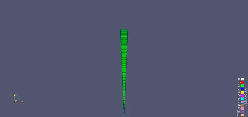
Mesh at the inlet of the pipe.

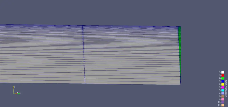
Mesh for the wedge side

Simulation:

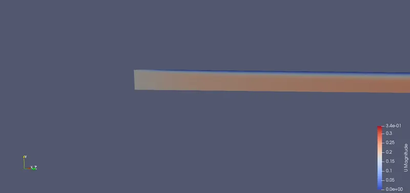
Velocity at the inlet of the pipe for 30th second.

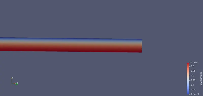
Velocity at the outlet for 30th second.

Pressure variation along the length of the pipe.

Output Graphs:

The plots shown below are for one half of the pipe.

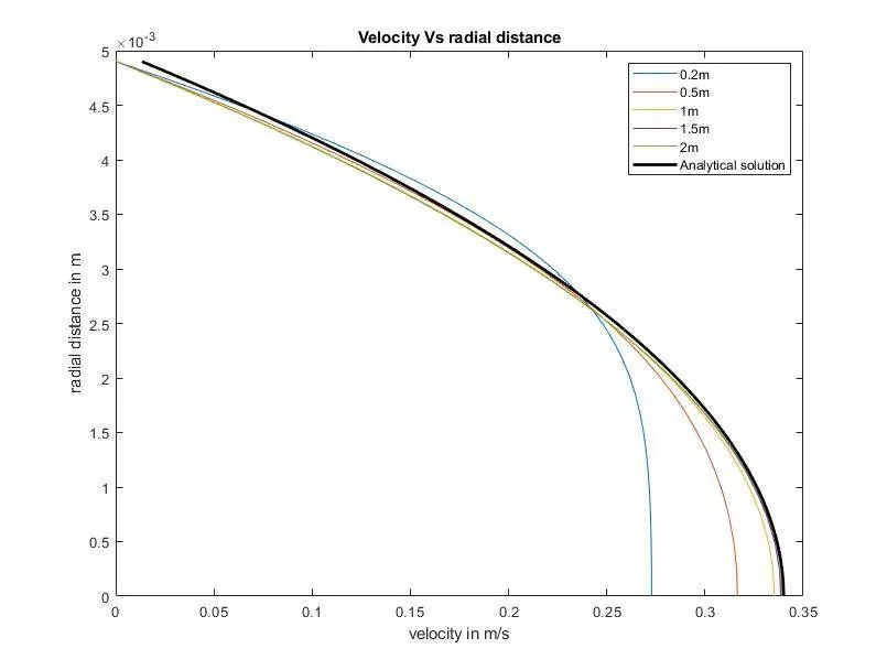
Velocity profiles at different locations along the length of the pipe.

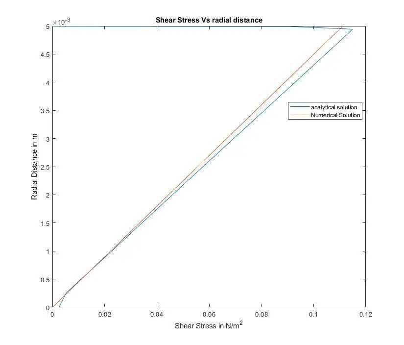
Shear stress comparisons of the numerical and analytical solutions.

Residual Plot.

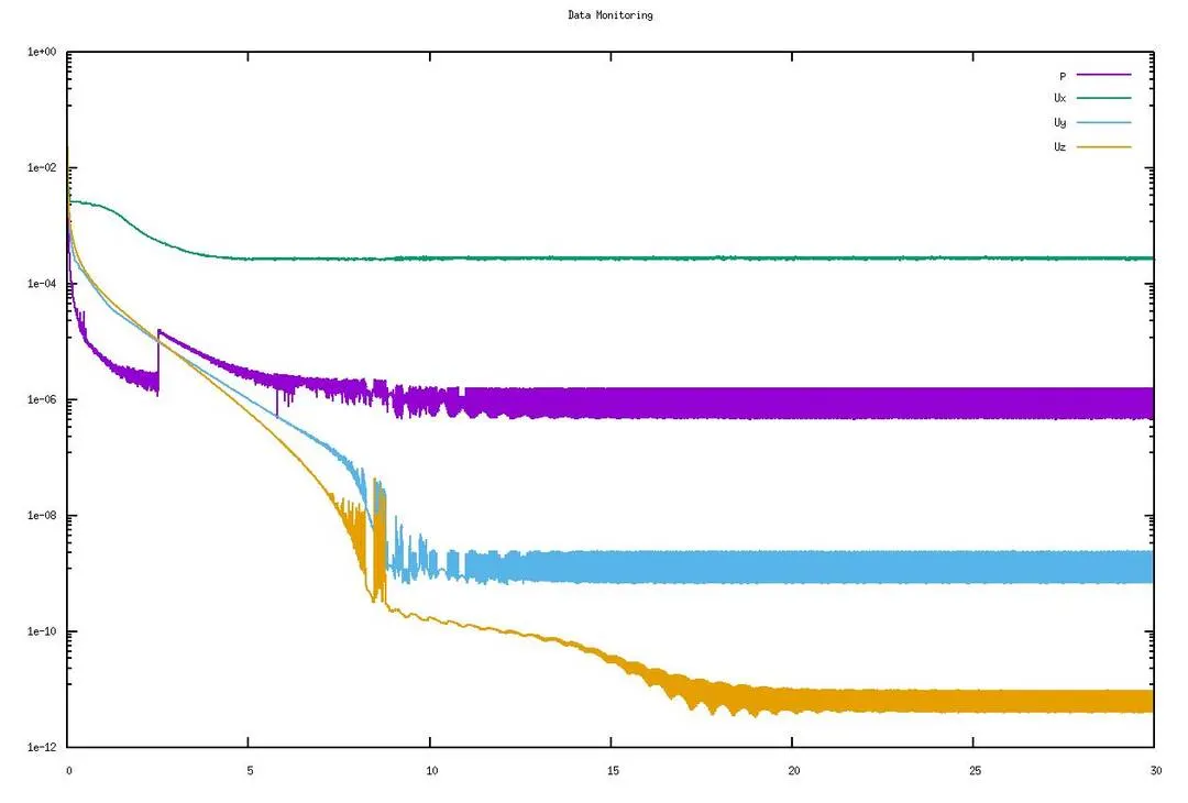
Explanation of the graph.

From the above plots, we can see that the numerical solution is close to the analytical solution. There is a small variation in numerical solution in the analytical solution this is because of the discretization error and the round-off error induced by the computer.

From the velocity plot, it can be inferred that the velocity is zero at the wall because of the velocity boundary layer and increases as the flow moves towards the center of the pipe.

From the shear stress plot, we can infer that the shear stress is maximum at the wall due to the viscosity of the fluid and decreases along the radial direction of the pipe, and is zero at the center of the pipe.

The residual plot is created to verify that the flow is fully developed for 30 second simulation time. As we can note that the residuals of the velocity and pressure are constant after 20 seconds. Hence with this plot, we can say that the flow reaches the steady-state after 20 seconds