Rayleigh Taylor Instability Challenge
Problem Statement:
1. Simulate the Rayleigh Taylor Instability analysis for two different mesh with a base mesh size of 0.5mm and compare the results with the help of simulation and explain the effect of mesh size on simulation.
2. Perform another simulation with water and user-defined material with density = 400kg/`m^3`, viscosity = 0.001 kg/m-s for the refined mesh.
3. Explain why the steady-state approach is not suitable for this type of simulation.
4. Define the Atwood number and find its values for case 1: water- air and Case 2: water-user defined material and explain its effect on the instability.
Introduction:
In multiphase flow, the parameters velocity, viscosity, pressure, and density are used to explain the movement of the fluid under the gravitational force. Rayleigh instability is hydrodynamic instability when a high-density fluid is placed over low-density fluid under the gravitational force. When the density interface is disturbed, the hydrostatic pressure is generated, so the heavier fluid moves downwards and mixes with the lighter one, with the amplitude of perturbation initially growing exponentially but after sometime saturates and forms the characteristic mushroom shape. When a heavier fluid is displaced downward with an equal volume of lighter fluid displaced upwards, it results in a decrease of potential energy than its initial state. This RTI has been applied to a wide range of problems including the mushroom clouds like volcanic eruptions, nuclear explosions, and plasma fusion reactors instability.
Richtmyer-Meshkov Instability (RMI).
RMI occurs when a shockwave is refracted by an interface between two materials. Shockwave creates an impulse that is sudden acceleration to the interface, RMI can be intuitively considered as a variant of RTI with an acceleration term.
Kelvin-Helmholtz Instability.
KHI occurs inflows with parallel velocity shear, with either homogeneous or heterogeneous fluid. In other words, KHI occurs when there is a velocity shear in a single continuous fluid or where there is a velocity difference across the interface between two fluids. At the late stage of RTI and RMI, the parallel velocity shear also rises between developed bubbles and spikes so KHI becomes relevant and generates the familiar mushroom cap-like seen in case of volcanic eruption, nuclear explosion, etc.
Saffman- Taylor Instability.
Saffman Taylor instability also known as viscous fingering is the formation of patterns in a morphologically unstable interface between two fluids in a porous medium. It occurs when a less viscous fluid is injected, displacing a more viscous fluid.
The same effect can be observed if the interface is horizontal and separates two fluids of different density and gravitational forces are acting on the two fluids. This effect is the same as RTI.
Saffman-Taylor Instability is seen often during drainage processes through media such as soils.
Salt Fingering.
Salt fingering is a mixing process that occurs when relatively warm, salty water overlies relatively colder, fresher water. It is driven by the fact that heated water diffuses more readily than salty water. A small parcel of warm, salty water sinking downwards into a colder, fresher region will lose its heat before losing its salt, making the parcel of water increasingly denser than the water around it and sinking further. Likewise, a small parcel of colder, fresher water will be displaced upwards and gain heat by diffusion from surrounding water, which will then make it lighter than the surrounding waters, and cause it to rise further. Paradoxically, the fact that salinity diffuses less readily than temperature means that salinity mixes more efficiently than temperature due to the turbulence caused by salt fingers.
Plateau-Rayleigh Instability.
Plateau- Rayleigh instability often called Rayleigh instability explains the reason for splitting the falling fluid into smaller packets with the same volume but less surface area. It is related to the Rayleigh Taylor Instability criteria. The main driving force for the Plateau-Rayleigh instability is that liquids by virtue of their surface tension which tend to minimize their surface area.
Atwood Number
It is the dimensionless number in fluid dynamics used in the study of hydrodynamic instabilities in density stratified flows.
`A = (rho_1 -rho_2)/(rho_1+rho_2)`
where
`rho_1` is density of heavier fluid.
`rho_2` is density of lighter fluid.
Geometry
Modeling of the geometry:
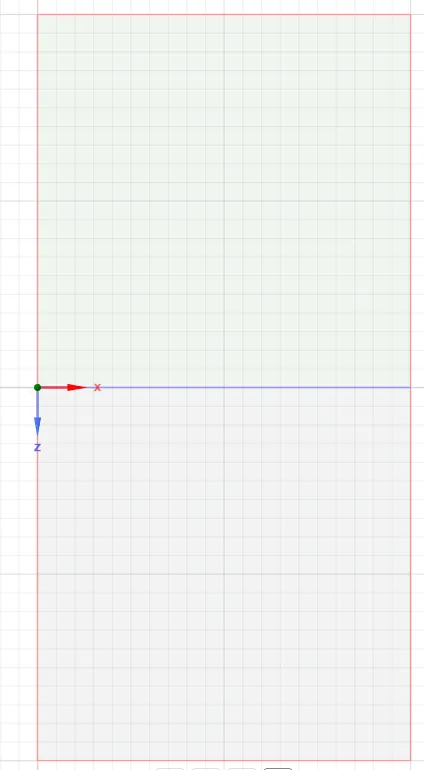
This simulation is done in 2D hence there is no need of creating any geometry in CAD software or importing any geometry. Simple geometry is created in SpaceClaim using the pull tool as shown in the figure. Share topology is given at the interface of the two fluids.
Meshing:
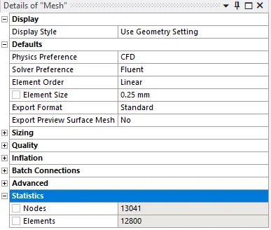
Mesh parameters for Case 1: Refined mesh.
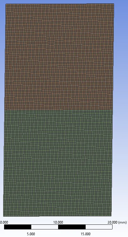
Meshed Model:
Setting Up physics in fluent:
1. Water material is added from the fluent database.
2. Pressure base solver is used.
3. Transient Solver is used to solve this case. Because at the early stage the instability is linear, as the simulation progresses the instability behaves non-linear.
4. Gravity is enabled in the negative y-direction. Because the RTI takes place in presence of the gravitational force.
5. Laminar model is chosen.
6. Multiphase->Volume Fraction is enabled with an implicit scheme. Because there are two fluids with different densities an implicit scheme is used as it unconditionally stable.
7. Patch is assigned with a volume fraction of 0 to lighter fluid, in this case, is air, and 1 for heavier fluid, in this case, is water.
8. SIMPLE scheme is used for pressure velocity coupling, for momentum, second-order upwind differencing scheme is used and for pressure, PRESTO is used. For transient formulation, a first-order implicit scheme is used as it stable and leads to an accurate solution.
Results:
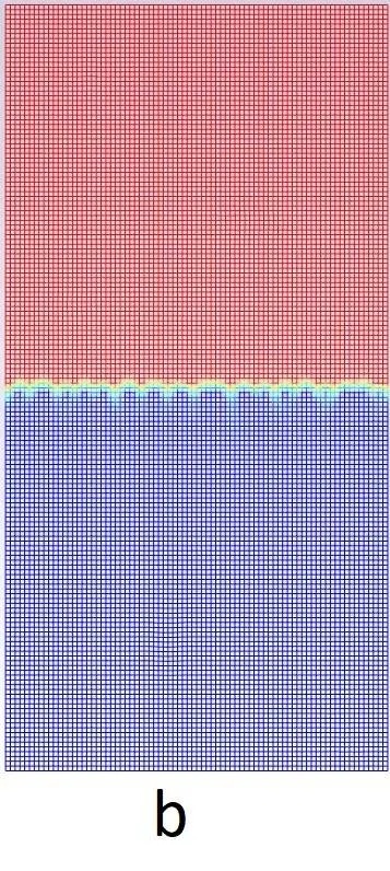
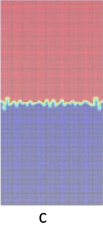
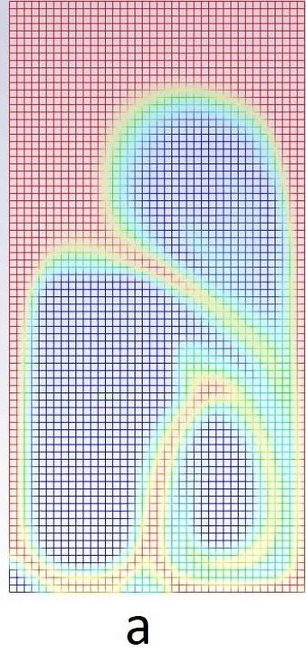
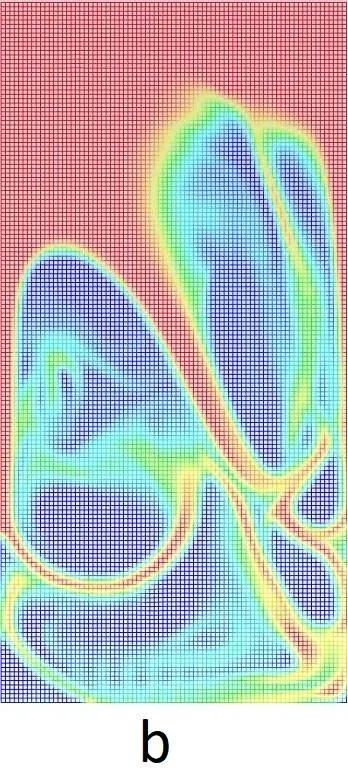
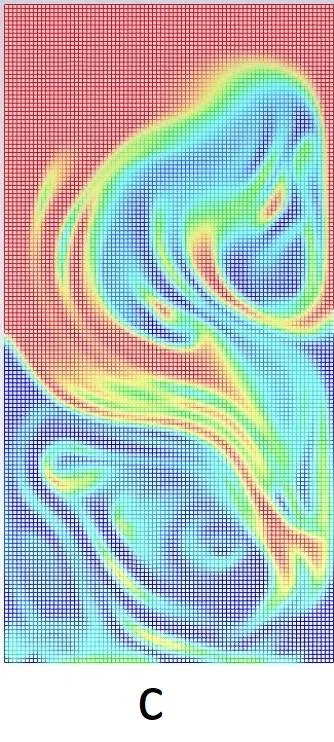
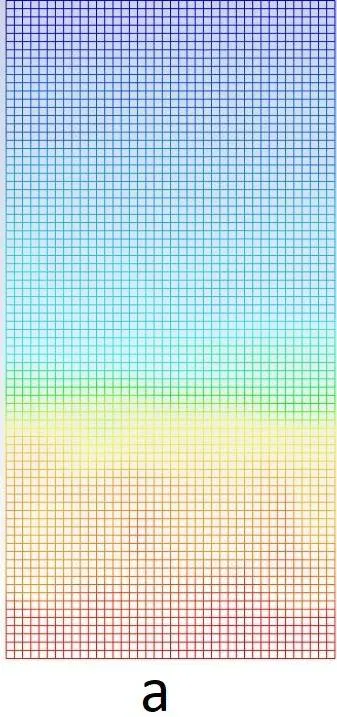
a: Base mesh
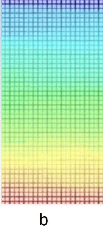
b: Refined mesh.
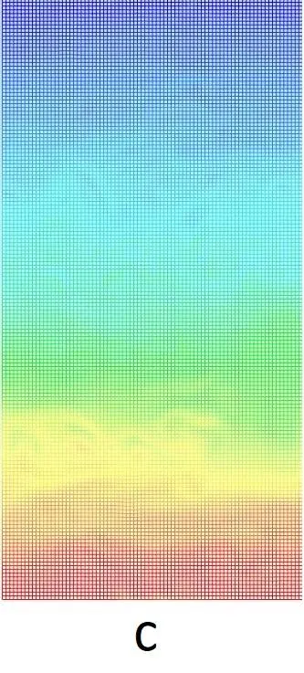
c: User-defined material
Plots representing the start of the instability.
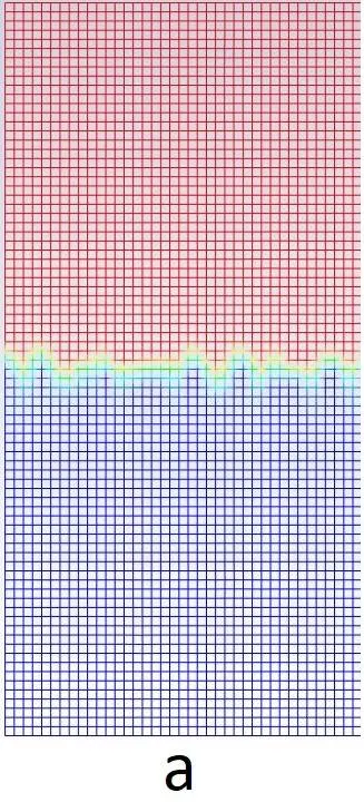
Plots at 350th iteration:
Plots after steady-state are achieved.
Simulation for a mesh size of 0.5mm with air and water:
Google drive link: https://drive.google.com/file/d/1pu_IwLwQK77OvFnpdaX_TK1gd-ReXl-4/view?usp=sharing
Simulation for a mesh size of 0.25 mm with air and water:
Google drive link: https://drive.google.com/file/d/1HYyFgEKmotae95wjNTFWMjo7zxAI7POD/view?usp=sharing
Simulation for a mesh size of 0.25 mm with water and user-defined material:
Google drive link: https://drive.google.com/file/d/1nsEn6ps2hGKnmYrG0EKABSp3vhfDXK9_/view?usp=sharing
Atwood Number for Water-air interface:
`rho` = 400kg/`,^3`.
`mu` = 0.001 kg/m-s.
`A = (rho_1 -rho_2)/(rho_1+rho_2)`
where
`rho_1` is density of water.
`rho_2` is density of air.
`A = (998.2-1.225)/(998.2+1.225) = 0.997`
Atwood Number for User defined material:
User defined material Properties:
`rho` = 400kg/`,^3`.
`mu` = 0.001 kg/m-s.
`A = (rho_1 -rho_2)/(rho_1+rho_2)`
where
`rho_1` is density of water.
`rho_2` is density of user defined material.
`A = (998.2-400)/(998.2+400) = 0.427`
Inference:
It is observed that the evolution of the interface grows faster with the increase in Atwood Number for which in this study the Atwood Number is kept as high as possible when using air and water. It was seen that with a larger Atwood Number, a larger amplitude of perturbations is observed. It is due to the larger density ratio of the two fluids, the stronger is the force to develop the interface instability. The Atwood Number is a dimensionless number in Fluid Dynamics. It is used in the study of the instabilities of the dynamics of the fluid flow. It gives the relation between the density of the higher fluid and the density of the lighter fluid.
With the decrease in Atwood Number from Case b to Case c and when compared, we can clearly observe from the contour plots that bubbles and spikes formation are still present at the same flow time or even after completion of simulation or at the verge of settling. The formation is because of the increase in density of secondary phase with a density of user-defined material
For the case of smaller Atwood Number, the density difference between the two sides of the interface are small and the density distribution of the upper and lower layers is nearly symmetrical. The initial density stratification plays a dominant role and the expansion compression effect has little influence. With the increased Atwood Number close to 1 the stabilization effect of initial density stratification decreases and the instability caused by the expansion-compression effect becomes more significant. It can be seen in the figures that the larger the Atwood numbers, the larger amplitude of perturbation. It takes place due to the larger density ratio of two fluids is, the stronger force to develop the interface instability. The flow structure of bubbles and globules are quite different both for the variation in meshing and also with the variation in Atwood Number. With the increase of Atwood number, the time of spikes or globules of the lighter phase fluid arriving at the bottom of the computational domain is accelerated, then the duration of RTI in the steady growth stage is shorter. We can observe that the compressibility on the bubble velocity is strong at a larger Atwood Number.
As the steady-state solution determines the fully developed solution and is not a time-accurate solution only the end results are obtained and as it is conditionally stable only smaller time steps should be used in order to satisfy the stability criteria. For transient simulation when compared to steady-state there is an increase in computational time. But as the transient solver implicit scheme is unconditionally stable smaller time steps can be used to run the simulations which enable to capture the flow accurately and observe the instabilities. Since the Transient solver is a time marching solution it is more accurate which makes it an ideal case set up to run the calculations for Rayleigh Taylor Instability analysis.