Project 2 - Rankine cycle Simulator

Introduction:

Rankine Cycle.

Rankine cycle is an idealized thermodynamic cycle of a heat engine that converts heat into mechanical work while undergoing phase change.

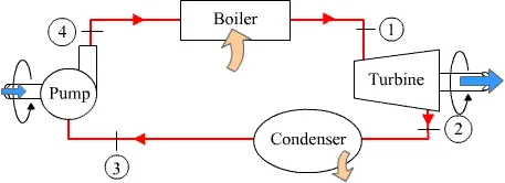
There are 4 phases

1. 1-2 Isentropic expansion in a pump.

The dry saturated vapour is expanded in the turbine generating power decreasing temperature and pressure and some condensation may occur. An isentropic process where entropy remains constant.

2. 2-3 Constant pressure heat rejection in condenser.

The working fluid from turbine with reduced pressure and temperature is sent to the condenser where heat is rejected at constant pressure. It is an isobaric heat rejection process.

3. 3-4 Isentropic compression in pump.

The working fluid with low pressure is pumped to high pressure with the help of pump to the boiler. It is an isentropic compression with constant entropy.

4. 4-1 Constant pressure heat addition in a boiler.

Heat is added to the high pressure working fluid by an external source to convert into superheated vapour.

Formulas:

1. Workdone in Turbine

`WDt = H1-H2` in KJ/Kg

where H1 and H2 represent enthalpy at state 1 and 2 respectively.

2. Work done by the pump

`WDp = V3*(P4-P3).100` in KJ/Kg

where V3 is specific volume at pressure P3

3. Efficiency

`eta = (1- ("Qrejected"/"Qadded")) *100` in %

Where Q rejcted is heat rejection between state points 2 to 3

4. Qadded is heat addition between state points 4 and 1

`Qadded = H1 - H4` in KJ

5. Qrejected is heat rejection between state points 2 and 3

`Qrejected = H2 - H3` in KJ

5. Specific Steam Consumption

`SSC = 3600/"WDnet"` KJ/KWh`

6. Back work ratio = `"WDp"/"WDt"`

Logic :

1. Code should ask for the user input.

2. To extract the required data from XSteam function to calculate the state points values.

3. Calculations for 4 state points using thermodynamic relations.

4. To calculate for the work done by turbine,pump, net work done, efficiency of the cycle and back work ratio using the formula.

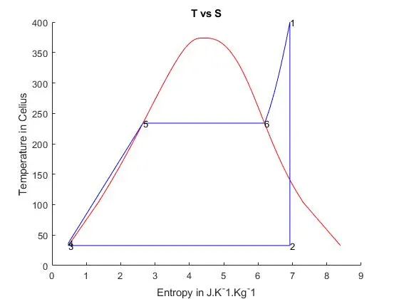
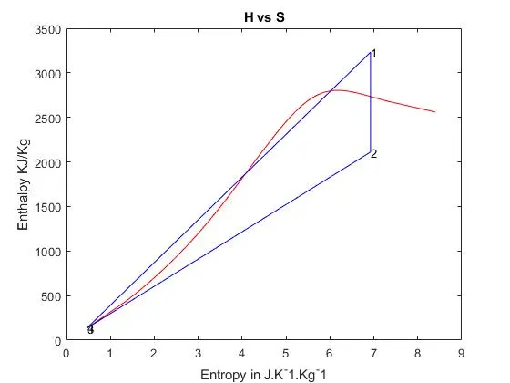
5. To plot the graph of TS and HS graph by first finding the temperature and entropy values between the user input pressure values. Similarly for HS graph

Main Script

close all
clear all
clc

%Displaying the cycles in the Rankine Cycle
disp ('Rankine cycle')
disp('1-2 Isentropic Expansion Process')
disp('2-3 Constant pressure heat rejection process')
disp('3-4 Isentropic compression Process')
disp('4-1 Constant pressure heat addition process')

%User input turbine inlet pressure, pump inlet pressure and turbine outlet
%temperature.
P1 = input('Enter the turbine inlet pressure(in bar):  ');
P2 = input ('Enter the condenser inlet pressure(in bar): ');
T1 = input ('Enter the temperature of turbine inlet (in Degree celius):  ');


%state point 1
%Function XSteam is called to extract entropy,enthalpy values corresponding
%to temperature and pressure
H1 = XSteam ('h_pT',P1,T1);
S1 = XSteam ('s_pT',P1,T1);

%state point 2

% From the graph S2=S1, P3=P2;
S2=S1;P3=P2;

%The specific entropy and specific enthalpy are extracted from the
%function and calculations are done with thermodynamic relations.
sf2 = XSteam('sL_p',P2);
sg2= XSteam('sV_p',P2);
sfg2 = sg2-sf2;
x = (S2-sf2)/sfg2;
hf2 = XSteam('hL_p',P2);
hg2 = XSteam('hV_p',P2);
hfg2 = hg2-hf2;
H2 = hf2+x*hfg2;
T3 = XSteam('Tsat_p',P3);
T2=T3;
S3 = XSteam('sL_p',P3);
H3 = XSteam('hL_p',P3);

S4=S3; P4=P1;
V3 = XSteam('vL_p',P3);
WDp = V3*(P4-P3)*100; %<-- Work done by the pump.

H4 = WDp+H3;
cp4 = XSteam('Cp_ps',P4,S4);
cv4 = XSteam('Cv_ps',P4,S4);
%finding in T4 using isentropic process formula
y = cp4/cv4;
r = (y-1)/y;
T4 = T3* (P4/P3)^r;

%work done by the turbine
WDt = H1-H2;

% heat rejection at constant pressure
Qrej = H2-H3;

%heat addition at constant pressure
Qadd = H1-H4;

% Net work done by the cycle
WDnet = WDt-WDp;
Back_work_ratio = WDp/WDt;

%Specific Steam Consumption
SSC = 3600/WDnet;

%efficiency of the cycle
n = (1-(Qrej/Qadd))*100;

% Calculation to plot staturation curve in TvsS curve and HvsS curve.

%pressure range for extracting temperature, entropy and enthalpy
prange= linspace(0.05,220,200);
for k = 1:200
    t_rangel(k) = XSteam('Tsat_p',prange(k));
    srange_l(k) = XSteam('sL_p',prange(k));
    hrange_1(k) = XSteam ('hL_p',prange(k));
end

prange= linspace(0.05,220,200);
for k = 1:200
    t_range2(k) =  XSteam('Tsat_p',prange(k));
    srange_2(k) = XSteam('sV_p',prange(k));
    hrange_2(k) = XSteam('hV_p',prange(k));

end

%Combine two matrices obtained from two for loops
%fliplr is used to flip the values such that the graph obtain is in correct
%format.
t_range = [t_rangel  fliplr(t_range2)];
srange = [srange_l fliplr(srange_2)];
h_range = [hrange_1 fliplr(hrange_2)];

%For loop to plot the graph between point 6 and point 1
temp0 = XSteam('Tsat_p',P1);

temp1 = linspace(temp0,T1,100);

for kk= 1 :length(temp1)
    
    tt(kk)= XSteam('s_pT',P1,temp1(kk));
end

%Extracting point 5 with XSteam function.
S5 = XSteam('sL_p',P1);
S6 = XSteam('sV_p',P1);

%Plotting the graph of T VS S graph
figure(1)
hold on
plot(srange,t_range,'color','r')
plot ([S1 S2 S3 S4 S5 S6 tt],[T1 T2 T3 T4 temp0 temp0 temp1],'color','b')
title('T vs S')
xlabel('Entropy in J.K^-1.Kg^-1')
ylabel('Temperature in Celius')
%Naming the state points 
text (S1, T1,'1')
text (S2, T2,'2')
text (S3, T3,'3')
text (S4, T4,'4')
text (S5, temp0,'5')
text (S6, temp0,'6')

%Plotting the graph H Vs S graph
figure(2)
plot (srange,h_range,'color','r')
hold on
plot ([S1 S2 S3 S4 S1],[H1 H2 H3 H4 H1],'color','b')
title('H vs S')
text (S1, H1,'1')
text (S2, H2,'2')
text (S3, H3,'3')
text (S4, H4,'4')
xlabel('Entropy in J.K^-1.Kg^-1')
ylabel('Enthalpy KJ/Kg')

%Displaying the Results
disp ('Results')
disp ('State Point 1')
fprintf ('P1 %.2f bar\n', P1)
fprintf ('H1 %.2f KJ/Kg\n', H1)
fprintf ('T1 %.2f Deg Celius\n', T1)
fprintf ('S1 %.2f J.K^-1.Kg^-1\n', S1)

disp('State Point 2')
fprintf ('P2 %.2f bar\n', P2)
fprintf ('H2 %.2f KJ/Kg\n', H2)
fprintf ('T2 %.2f Deg Celius\n', T2)
fprintf ('S2 %.2f J.K^-1.Kg^-1\n', S2)

disp('State Point 3')
fprintf ('P3 %.2f bar\n', P3)
fprintf ('H3 %.2f KJ/Kg\n', H3)
fprintf ('T3 %.2f Deg Celius\n', T3)
fprintf ('H3 %.2f J.K^-1.Kg^-1\n', H3)

disp('State Point 4')
fprintf ('P4 %.2f bar\n', P4)
fprintf ('H4 %.2f KJ/Kg\n', H4)
fprintf ('T4 %.2f Deg Celius\n', T4)
fprintf ('S4 %.2f J.K^-1.Kg^-1\n', S4)

fprintf('Work done by pump %.2f KJ/Kg\n', WDp)
fprintf('Word done by turbine %.2f KJ/Kg\n', WDt)
fprintf('Heat rejected %.2f KJ\n ', Qrej)
fprintf('Heat addition %.2f KJ\n', Qadd)
fprintf('Net work done %.2f KJ/Kg\n', WDnet)
fprintf('Efficiency %.2f percent\n', n)
fprintf('Back work ratio %f\n', Back_work_ratio)
fprintf('SSC %f KJ/ KWh\n', SSC)

Explanation.

disp ('Rankine cycle')
disp('1-2 Isentropic Expansion Process')
disp('2-3 Constant pressure heat rejection process')
disp('3-4 Isentropic compression Process')
disp('4-1 Constant pressure heat addition process')

This code displays the phases of rankine cycle so that user will know what are the state points and to input correct pressure and temperature values.

P1 = input('Enter the turbine inlet pressure(in bar): ');
P2 = input ('Enter the condenser inlet pressure(in bar): ');
T1 = input ('Enter the temperature of turbine inlet (in Degree celius): ');

This code asks the user to input the turbine and condenser inlet pressure in bar and temperature at the turbin inlet in degree celius.

From the given inputs

H,S,T,P for the 4 state points are calculated.

At state point 1

Enthalpy is found from Xsteam as function of pressure and temperature and similary for enthropy as well.

At State point 2

Saturated entropy and enthalpy sf2,sg2,hf2,hg2 are extracted as a function of pressure P2.

Since P3=P2;

temperature of state point 3 is extracted from steam table as function of pressure P3.

With Saturated entropy and enthapy known H2,S2 are calculated and dryness fraction is found out.

S3 and H3 is extracted from steam table function as a function of P3.

V3 is specific volume which is also extracted as a function of P3.

WD by the pump is calculated using the above mentioned formula.

With calculation of Work done by the pump H4 is calculated.

T4 is calculated with isentropic process formula.

With all the state point variables found Workdone by the turbine, efficiency, net work done, specific steam consumption,heat addition and rejection are calculated.

For plotting of the saturation curve

Saturated temperature and entropy are extracted as a function of pressure. Hence a for loop is created for a pressure range.

Hence graph is plotted for saturation curve and all the state points and each state points are represented with 1,2,3,4 values respectivly.

Output: