Week 3 - Solving second order ODEs

1. Introduction

An ordinary differential equation (ODE) is a mathematical function consisting of essentially one independent variable and its relation with respect to its derivatives. Examples of ODEs to describe physical phenomena and applications include Newton's law of cooling in packaging industry with the consumable contents initially subjected to high temperatures before being allowed to cool for packaging reasons and radioactive decay to find half-life of radioactive elements such as use of Cobalt-60 to emit gamma rays for cancer treatment requires regular replacement for better effectiveness, to name a few. ODEs can be distinguished as linear or non-linear, homogeneous or inhomogeneous, and constant coefficients or variable coefficients. The aim of this programming exercise was to solve a second order ODE representing a simple pendulum motion with damping and the pendulum's movement depending on Newtons second law.

2. Method

2.1 Modelling

The problem was solved by building a mathematical model in Python using the Sublime Text source code editor (code snippet for which is attached with this report) along with the math, numpy and matplotlib.pyplot modules/libraries for defining mathematical expressions, creating arrays and its corresponding expressions, and building the concerned plots respectively. Since, the ODE is second order with constant coefficients, the choice of solver for calculation was chosen as odeint from the scipy.integrate package which essentially uses lsoda algorithm from the FORTRAN library odepack and consists of mainly three inputs viz., Function name which returns derivative values for given y and t values, Initial conditions, and time intervals. Additional arguments can be passed to define certain inputs that may be utilised for the particular function name. It should be noted that the second order ODE for the given problem needs to be converted to a system of first order ODEs for odeint to perform the necessary calculations. The conversion of the same has been explained in detail in Section 2.2 of this report.

2.2 Mathematical Model Setup

Function, `f(theta) = (d^2theta)/(dt^2) + (b/m)*(d theta)/(dt) + (g/L)*sin theta = 0` (1)

Conversion of Function to system of first order ODEs:

Let `theta_1 = theta`, and (2)

`theta_2 = (d theta_1)/(dt)`. Then, (3)

`(d^2 theta)/(dt^2) = (d^2 theta_1)/(dt^2) = (d theta_2)/(dt)` (4)

Substituting eq. (2), eq. (3) and eq.(4) in eq. (1) results in:

`(d theta_2)/(dt) + (b/m)*(d theta_1)/(dt) + (g/L)*sin theta_1 = 0`

OR

`(d theta_2)/(dt) + (b/m)*theta_2 + (g/L)*sin theta_1 = 0` (5)

From eq. (3) and eq. (5), it is realised

`theta_2 = (d theta_1)/(dt)`, and

`(d theta_2)/(dt) = − (b/m)*theta_2 − (g/L) sin theta_1`

The above equations can be represented in an equivalent matrix form as shown below:

`[ [(d theta_1)/(dt)], [(d theta_2)/(dt)] ] = [ [theta_2], [− (g/L)*sin theta_1 − (b/m)*theta_2] ]` (6)

Eq.(6) represents matrix of 2 rows and 1 column on either side of the equality sign indicating a solution is possible and this has been represented in the function named model within the Python program and is solved using values of given constant coefficients as well as initial conditions of time, and angular displacement and angular velocity starting at time, t = 0, by passing it as arguments for the odeint function. The initial conditions and constant coefficient values have been declared in the main Python program as it allows for better control in terms of variation in the same values. The resulting values obtained from the solution of the odeint function represents the values of angular displacement and angular velocity at the selected time intervals.

2.3 Post-Processing

In addition to the solution of the given ODE for the initial conditions of time for a timespan from 0 to 20 seconds and values of the damping coefficient, gravity, length of the pendulum and mass of the ball, shapes such as rectangle, circle and arrows have been made use of by accessing the matplotlib.patches.Rectangle class, matplotlib.patches.Circle class and matplotlib.pyplot.arrow() function respectively, to create different geometries such as bob, pivot and brick layers with the pendulum rod created using normal line plot function in order to simulate the simple pendulum motion. The motion has been captured as images with the filenames saved with the expression, "str(round(i/len(t),5))" where 'i' indicates the value of time at that instant and 'len(t)' representing the length of time array, as this format was easily recognised by the ImageMagick software during stitching of all the images, as it progresses from the smallest value to the largest value without missing any file in between, into a '.gif' file which can be viewed in Section 3, Results. Legends, titles, x labels, and y labels have been added for a better understanding of the graphical representations.

3. Results

3.1 Computed values of Angular Displacement and Angular Velocity

Fig.1 and Fig. 2 below captioned 'Plot of Angular Displacement vs Time' and 'Plot of Angular Velocity vs Time' respectively, shows the values computed for Angular Displacement and Angular Velocity at different time intervals using the odeint function. The values were calculated using the method adopted to convert second order ODE to a system of first order ODEs as was explained in subsection 2.2, Mathematical Model Setup. It can be seen from the respective figures that although they have diminishing amplitudes over the timespan of 20 seconds, their starting points are different. This can be reasoned on the grounds that the ODE represents the equation of motion in which angular displacement is an indicative of the derivative of change in position of the Bob with regards to time while angular velocity denotes change in velocity of the Bob, again with respect to time, and also with both having different initial values at time, t = 0. Additionally, angular displacement gets further reduced due to the influence of the damping coefficient.

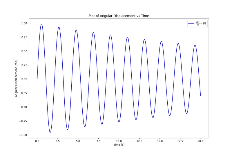
Fig. 1: Plot of Angular Displacement vs Time

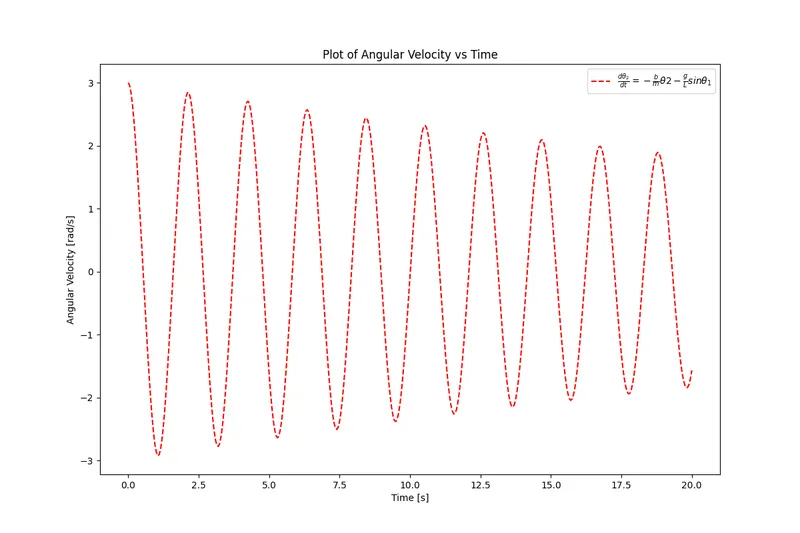
Fig. 2: Plot of Angular Velocity vs Time

3.2 Simple Pendulum animation

In the '.gif' file attached below, the motion of simple pendulum has been converted from the images obtained to an animation as was mentioned previously in subsection 2.3 Post-Processing. The animation demonstrates maximum displacement of the pendulum to the extreme left and right positions based on the corresponding peak angular displacement values it achieves when compared with Fig. 1 (trough and crest position of each 'wave'). However, at that very instant, angular velocity values at those extreme positions reach at nearly 0 and consequently, attain their maximum values whenever angular displacement nears 0. This behaviour revisits an already addressed fact about the nature of the ODE as stated in subsection 3.1, Computed values of Angular Displacement and Angular Velocity.

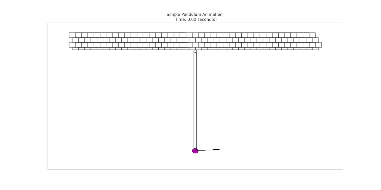
Fig. 3: Animation of a simple pendulum

4. Discussion

The given second order ODE evaluation using odeint function highlights the capabilities of calculating angular displacement and angular velocity values between the time range of 0 and 20 seconds through the lsoda algorithm incorporating the Adams method for a non-stiff ODE as can be seen from the results displayed in Fig. 1 and Fig. 2 where the solutions obtained are not changing by large orders of magnitudes. The lsoda algorithm initially uses the non-stiff method and dynamically monitors data in order to decide if it needs to continue with this approach or change it.

5. Conclusion

Solution for the given second order ODE through the odeint function in Python using the Sublime Text source code editor was well understood with this programming exercise. It was realised that depending on the timespan, initial conditions and coefficient values of different system related variables, it was possible to determine the values of angular displacement and angular velocity, through the lsoda algorithm of the odeint function. Also, with regards to the solution obtained and the visual representation of the simple pendulum motion greatly assisted in appreciating the importance of understanding the benefits of mathematical solutions to physical applications.

CODE:

Program to solve second order Ordinary Differential Equation (ODE) that defines transient behaviour of a pendulum using the odeint function from the scipy.integrate package.

# Program to simulate the simple pendulum motion
# Author: Diptesh Pawa

# Modules/Libraries
import math
import matplotlib.pyplot as plt
import numpy as np
from scipy.integrate import odeint
import matplotlib.patches as patches
from matplotlib.patches import Rectangle, Arrow

# Function to calculate dz/dt
def model(theta,t,b,g,l,m):
	theta1 = theta[0]
	theta2 = theta[1]
	dtheta1_dt = theta2
	dtheta2_dt = -(b/m)*theta2 - (g/l)*math.sin(theta1)
	dtheta_dt = [dtheta1_dt, dtheta2_dt]
	return dtheta_dt

# Inputs
b = 0.05  # Damping coefficient
g = 9.81  # Gravity [m/s^2]
l = 1     # Length of the pendulum [m]
m = 1 	  # Mass of the ball [kg]

# Initial condition
theta_0 = [0,3]

# Time dataset
dt = 0.05
t = np.arange(0,20+dt,dt)
print('t = ', t)

# Outputs
# Solve ODE
theta = odeint(model, theta_0, t, args=(b,g,l,m))

# Plotting of angular displacement and angular velocity curves
fig_1 = plt.figure(figsize=(12, 8))
ax = fig_1.add_subplot(111)
ode_1 = ax.plot(t, theta[:,0], 'b-', label=r'$\frac{d\theta_1}{dt}=\theta2$')
ax.set_ylabel('Angular Displacement [rad]')
ax.set_xlabel('Time [s]')
plt.legend(loc='best')
plt.title("Plot of Angular Displacement vs Time")
plt.savefig('Week_3_ang_disp_time.png')

fig_2 = plt.figure(figsize=(12, 8))
ax_2 = fig_2.add_subplot(111)
ode_2 = ax_2.plot(t, theta[:,1], 'r--', label=r'$\frac{d\theta_2}{dt}=-\frac{b}{m}\theta2-\frac{g}{L}sin\theta_1$')
ax_2.set_ylabel('Angular Velocity [rad/s]')
ax_2.set_xlabel('Time [s]')
plt.legend(loc='best')
plt.title("Plot of Angular Velocity vs Time")
plt.savefig('Week_3_ang_vel_time.png')

# Origin
O = [0,0]

# Dimensions of objects to be drawn as part of the simple pendulum animation
Brick_length = 0.05;
Pivot_radius = 0.0125
Bob_radius = 0.025

# Defining plot, subplots and Axes limits
fig_3, ax_3 = plt.subplots(figsize=(16, 8))
limits = 1.2*l;
ax_3.set_xlim(-limits, limits)
ax_3.set_ylim(-limits, limits/4)
currentAxis = plt.gca()
line, = ax_3.plot([], [], 'o-', linewidth=2, color = "black")

# Creating different layers of bricks
for i in range(1,20):
	# Wall Layer
	currentAxis.add_patch(Rectangle(((O[0]-Brick_length*(i+1)), (O[1]+Brick_length/2)), Brick_length*2, Brick_length/2, fill=None, alpha=1))
	currentAxis.add_patch(Rectangle(((O[0]+Brick_length*(i-1)), (O[1]+Brick_length/2)), Brick_length*2, Brick_length/2, fill=None, alpha=1))
	
	# First Layer of Bricks
	currentAxis.add_patch(Rectangle(((O[0]-Brick_length*(i+1.5)), (O[1]+Brick_length)), Brick_length*2, Brick_length, fill=None, alpha=1))
	currentAxis.add_patch(Rectangle(((O[0]+Brick_length*(i-0.5)), (O[1]+Brick_length)), Brick_length*2, Brick_length, fill=None, alpha=1))
	
	# Second Layer of Bricks
	currentAxis.add_patch(Rectangle(((O[0]-Brick_length*(i+1)), (O[1]+(Brick_length*2))), Brick_length*2, Brick_length, fill=None, alpha=1))
	currentAxis.add_patch(Rectangle(((O[0]+Brick_length*(i-1)), (O[1]+(Brick_length*2))), Brick_length*2, Brick_length, fill=None, alpha=1))
	
	# Third Layer of Bricks
	currentAxis.add_patch(Rectangle(((O[0]-Brick_length*(i+1.5)), (O[1]+(Brick_length*3))), Brick_length*2, Brick_length, fill=None, alpha=1))
	currentAxis.add_patch(Rectangle(((O[0]+Brick_length*(i-1.5)), (O[1]+(Brick_length*3))), Brick_length*2, Brick_length, fill=None, alpha=1))

# Locating pivot point
Pivot = currentAxis.add_patch(plt.Circle((O[0], O[0]+(Pivot_radius/1.5)), Pivot_radius, fill = False))

# Disabling x-axis and y-axis ticks
currentAxis.axes.get_xaxis().set_ticks([])
currentAxis.axes.get_yaxis().set_ticks([])

# Simulating pendulum motion
for i in range (0,len(t)):
	
	# Defining X and Y coordinates of the Bob
	Xcoord=[0,l*math.sin(theta[i,0])]
	Ycoord=[0,-l*math.cos(theta[i,0])]
        
    # Locating Mass Point
	MP = [Xcoord[1], Ycoord[1]]

	# Pendulum
	Rod_1 = ax_3.plot([(O[0]-(Pivot_radius)),(MP[0]-(Pivot_radius))], [O[1], MP[1]], linewidth=2, color = 'black')
	Rod_2 = ax_3.plot([(O[0]+(Pivot_radius)),(MP[0]+(Pivot_radius))], [O[1], MP[1]], linewidth=2, color = 'black')
	     
	# Bob
	Bob = currentAxis.add_patch(plt.Circle(((MP[0]), (MP[1]-(Bob_radius/2))), Bob_radius, ec = 'k', facecolor='m'))
	
	# Circle at Mass Point
	MP_circle = currentAxis.add_patch(plt.Circle(((MP[0]), (MP[1]-(Bob_radius/2))), Pivot_radius/5, fill=None, alpha=1))
    
	plt.title("Simple Pendulum Animation \n Time: %0.2f second(s)" % (i*dt))
	
	# Arrow to indicate pendulum motion
	if i<len(t)-1:
		x_1 = [MP[0], l*math.sin(theta[i+1,0])]
		y_1 = [MP[1], -l*math.cos(theta[i+1,0])]
		
	drawArrow = plt.arrow(x=Xcoord[1], y=(Ycoord[1]-(Bob_radius/2)), dx=(x_1[1]-x_1[0]), dy=(y_1[1]-y_1[0]), head_width=0.01, head_length=0.05, fc='k', ec='k')

	# Saving images at each time instant based on the sizing interval
	filename = str(round(i/len(t),5)) + '.png'
	
	plt.savefig(filename)

	# Copying the last values for the two Rods drawn previously before removing them.
	line_1 = Rod_1.pop(0)
	line_2 = Rod_2.pop(0)
	
	if i<len(t):
		
		drawArrow.remove()
		Bob.remove()
		MP_circle.remove()
		line_1.remove()
		line_2.remove()
	
plt.show()