Steady Vs Unsteady flow over a cylinder

1. Introduction

Flow around objects exists from commonly observed movement of animals in nature such as the flight of birds ranging from the smallest in size to the largest to man-made applications viz., in heat exchangers, chimney stacks, and commercial and cargo flight aircrafts respectively and a growing significance to understand the different fluid flow phenomena like lift and drag coefficients, boundary layer separation, vortex shedding, etc., has been extensively exploited in recent years and in many cases to solve existing issues with the previously mentioned engineering applications. One such peculiar interest that gained importance over time was the flow around a circular cylinder and more specifically to comprehend the phenomenon of Karman vortex street which is when the wake behind the circular cylinder becomes unstable beyond a certain value of Reynolds number.

The aim of this challenge is to perform steady-state simulations using laminar viscous model for Reynolds number 10 and 100 while a steady-state solver and turbulence model was investigated for Reynolds number 1000, 10000 and 100000 in ANSYS Fluent 2020 R1, owing to the nature of wake behaviour observed from initial experimental findings by Roshko & Fiszdon in 1969 [1] and later updated by Roshko in 1993 [2], to calculate the coefficient of drag and lift by varying the velocity of the flow. Additionally, transient simulations using laminar viscous model to determine the Strouhal Number based on the frequency of vortex shedding for Reynolds number 100 was performed. The analysis involves verification of the computed results with a mesh independence study for Reynolds number 10 and 100 detailing on the mesh refinement approach that would outline cell count, coefficient of drag values and number of iterations for convergence for each mesh based on stability of behaviour for monitor points, plots indicating development of vortex shedding behind the cylinder as well as some of the mesh quality attributes like element quality, skewness, orthogonality, and aspect ratio. A refined mesh setup for Reynolds number 1000, 10000 and 100000 was created based on the 'y+' value, boundary layer thickness and required number of inflation layers to capture the boundary layer flow properties. In both cases of mesh development, the results for coefficient of drag have also been validated by limiting the error within 5 % difference against experimental values.

2. Method

2.1 Modelling

The computational domain for simulating flow around a circular cylinder was modelled in SpaceClaim, the default solid modeling CAD software for the Fluid Flow (Fluent) Analysis System. Since, the computational domain has a uniform input flow of constant magnitude in all directions defined in a two-dimensional space, the simulations were carried out for one half of the model along the spanwise symmetry plane i.e., the model size was reduced for a faster computational time. The diameter (D) of the circular cylinder is set at 2m created using the 'Circle' option in the 'Sketch' menu under the 'Design' tab. The inlet side of the computational domain is defined at 10D while the outlet at 20D, both from the centre of the cylinder which was outlined using construction lines. The height of the inlet and outlet sides is set at 10D after which a rectangle from the 'Rectangle' tool in the 'Sketch' menu under the 'Design' tab was used to define the extent and region of the computational domain. In order to perform discretization and define the physical boundaries, a surface was required to be created from the given measurements. SpaceClaim offers a feature called the 'Pull' tool in the 'Edit' menu of the 'Design' tab which will highlight the entire domain by changing the colour indicating that the surface has been created. The circular area and construction lines can now be deleted while also ensuring that the rendered area and the centre of the cylinder remains unaffected. Also, we make a note of the cylinder diameter which will be used to define the monitor point to identify the velocity behaviour in the solution and post-processing step.

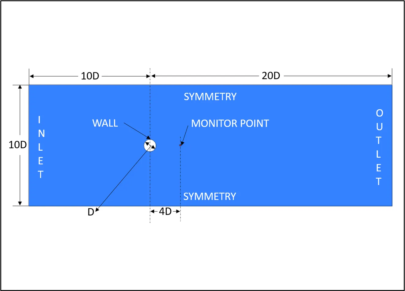
Fig. 1: Fluid Volume Model, Boundary Conditions regions and Monitor Point at a distance of four times the diameter of the cylinder upstream from its centre (D = 2m)

2.2 Meshing

The meshing approach adopted for the given computational domain was developed to maintain the meshing quality attributes viz., element quality, skewness, orthogonality, and aspect ratio within the ranges as laid out in the Meshing training material of ANSYS outlined in the following table:

Element Quality			0 (Bad Mesh)	1 (Good Mesh)
Aspect Ratio		Triangles	1 (for an equilateral triangle)	- Best possible value
		Quadrilaterals	1 (for a square)	- Best possible value
Skewness	0-0.25 (Excellent)	0.25-0.50 (Very Good)	0.50-0.80 (Good)	0.80-0.94 (Acceptable)	0.95-0.97 (Bad)	0.98-1.00 (Unacceptable)
Orthogonal Quality	0-0.001 (Unacceptable)	0.001-0.14 (Bad)	0.15-0.20 (Acceptable)	0.20-0.69 (Good)	0.70-0.95 (Very Good)	0.95-1.00 (Excellent)

Table 1: Mesh Quality Attributes as defined in the ANSYS meshing training material

The reason for pursuing the mesh quality attributes outlined in Table 1 is based on the fact that across different types of geometries/models, these are few of the known ways of identifying whether the discretized mesh is likely to have convergence issues during the solution process and also to locate areas in the mesh where the statistics can be improved. For each of the mesh, named selections such as inlet, outlet, symmetry and walls have been created so as to assign their respective boundary conditions in the setup stage. Also, depending on the name of the named selection, Fluent is able to assign an inlet, outlet, symmetry or wall boundary condition with velocity-inlet, pressure-outlet, symmetry and wall type boundary conditions respectively which is a useful feature to have in flow-type problems of similar nature since the user now can only add values relating to the specific boundary condition thereby making the setup process a lot faster. In Section 2.5.1, we will discuss in detail about the different meshes that were prepared, their mesh qualities and the arrival on mesh independent solution while in Section 2.5.2, the process on mesh refinement with regards to the boundary layer development and turbulence model of choice will be described.

2.3 CFD Simulation Setup, Boundary Conditions, Monitoring Points and Solution

The simulations on all meshes for Reynolds number 10 and 100 was performed using the Laminar viscous model while for Reynolds number 1000, 10000 and 100000, the Reynolds Averaged Navier-Stokes (RANS) models i.e, the k-`omega` turbulence models approach was used. The use of turbulence model for Reynolds number 1000 and above is attributed to the early investigations and measurements carried out on the flow regimes (Roshko & Fiszdon, 1969 [1]) and (Roshko, 1993 [2]), where the vortex formation in the near wake of the cylinder exhibited a transition from a steady and laminar vortex street to an unsteady and turbulent vortex street while still maintaining a laminar boundary layer around the object. Additionally, all simulations are being run using the double-precision feature to accurately measure the prediction quantities (coefficient of drag and lift) especially due to the different Reynolds number and as a general measure to resolve large variations in pressure differences. A brief description into the working of the Laminar viscous model and k-`omega` turbulence model is provided below:

2.3.1 Laminar viscous model

The Laminar viscous model can be described as the solution of the governing fluid equation viz., Navier-Stokes equations for a domain, in this case, discretized using the finite volume approach, without the presence of turbulence terms. The Navier-Stokes equations define the fluid flow properties such as velocity, pressure, density, temperature, viscosity, energy, etc., within a given physical domain. Additionally, the Navier-Stokes equations are developed with regards to the laws of conservation that states the net mass flow across a system is zero (Conservation of mass) and that the momentum within the same system (or control volume) is constant (Conservation of momentum). If energy is also a variable of assessment for the given domain, then according to the first law of thermodynamics, total heat gain of a system is equal to the sum of heat added to the system and work done on the same system.

For the given problem, the computational domain is two-dimensional and energy is not a variable of assessment. This implies that the Navier-Stokes equations that will be solved using the Laminar viscous model is for the conservation of mass or continuity equation and conservation of momentum.

2.3.1.1 Setup of the Laminar viscous model:

To use the Laminar viscous model in the Fluent component system, we navigate to Viscous option in Models under the Physics Tab. In the Viscous Model feature window, we choose Laminar as the option.

2.3.2 k-`omega` turbulence model

The k-`omega` turbulence model consists of two transport equations to measure the convection and diffusion properties of turbulent energy viz., the turbulent kinetic energy (k) term, similar to the one in the k-`epsilon` turbulence models, to evaluate the energy in turbulence and `omega` to determine the turbulence scale. The `omega` equation in the standard k-`omega` turbulence model has a major downside in the form of a high sensitivity of the solution dependent on the freestream values of k and `omega` outside the shear layer. This drawback has been addressed particularly well by the k-`omega` SST turbulence model wherein it combines terms of the `omega` and `epsilon` equation. Within the freestream, the k-`omega` SST turbulence model makes use of the `epsilon` equation which is where the `omega` equation is most sensitive to while in the rest of the region the `omega` equation is made use of. This switching behaviour of the k-`omega` SST turbulence model makes it particularly effective in dealing with adverse pressure gradient and separating flow related applications. Also, when compared with the k-`epsilon` turbulence model, the effects of turbulence in stagnation and strong acceleration zones are relatively smaller. The SST model in the k-`omega` SST turbulence model deals with the calculation of the principal shear stress in adverse pressure gradient boundary layers.

2.3.2.1 Setup of the k-`omega` SST turbulence model:

The k-`omega` model is available in the Model section of Viscous Model feature and when we choose the SST option in the type, we now set the k-`omega` model' to 'k-`omega` SST turbulence model. Production limiter in the options section is an option selected by default and essentially limits the generation of excessive turbulence energy around stagnation points.

2.3.3 Boundary Conditions and Monitoring Points

The different boundary conditions for the simulation of flow over a cylinder is described in the following table:

Named Selections	Inlet	Symmetry	Walls	Outlet
Type	Velocity-inlet	symmetry	wall	pressure-outlet
Velocity Specification Method	Magnitude, Normal to Boundary	--	--	--
Velocity Magnitude (m/s)	0.25 (Reynolds number 10)	--	--	--
	2.5 (Reynolds number 100)	--	--	--
	25 (Reynolds number 1000)	--	--	--
	250 (Reynolds number 10000)	--	--	--
	2500 (Reynolds number 100000)	--	--	--
Turbulence Specification Method	Intensity and Viscosity Ratio	--	--	--
Turbulent Intensity (%)	5	--	--	--
Turbulent Viscosity Ratio	10	--	--	--
Gauge Pressure (Pa)	--	--	--	0
Wall Motion	--	--	stationary wall	--
Shear Condition	--	--	no slip	--

Table 2: Boundary Conditions including different velocity values for simulation of flow over a cylinder

For the given problem, the material properties are different from the standard and available materials in the Fluent database for which we head over to the 'Create/Edit' button in the 'Materials' section of the 'Physics' tab and click on it to open the 'Create/Edit Materials' window. To create a user-defined material, we begin by selecting 'air' as the base material from the 'Fluent Database' and click on the 'Copy' button followed by assigning a name, in this case 'user_material'. In order to assign the 'user_material', we need to select the 'Cell Zones' option under the 'Zones' section of the 'Physics' Tab and choose 'fff_surface' which represents the fluid volume. After the 'fff_surface' has been highlighted in the 'Cell Zone Conditions' window, we can click on the 'Edit' button and select 'user_material' from the 'Material Name' drop-down list followed by clicking on the 'OK' button. Thereafter, we can head back over and click on the 'Create/Edit' button in the 'Materials' section of the 'Physics' tab to delete 'air' and/or any other material from the 'Fluent Fluid Materials' drop-down menu. In the same 'Create/Edit Materials' window, the Density value is changed to 1 `(kg)/m^3`and the Viscosity (or dynamic viscosity) value to 0.05 `(kg)/(ms)`. The velocity values in Table 2 are defined with respect to the Reynolds number calculations based on the 'user_material' density and viscosity values.

The choice of Turbulence specification method chosen for this simulation is Intensity and Viscosity Ratio wherein the Intensity (or Turbulent Intensity) is defined as the ratio of root-mean-square (RMS) value of velocity fluctuations to average flow velocity while Viscosity Ratio (or Turbulent Viscosity Ratio) is defined as the ratio of the turbulent viscosity to the laminar viscosity. Turbulent intensity is set to its default value of 5% (representing medium intensity) and the Turbulent Viscosity Ratio has its default value at 10 since the values for the same are not directly available and in that case, for an external flow simulation, these values usually lie in a typically good scale or range as is recommended in Lecture 3. Turbulence Modeling, Heat Transfer & Transient Calculations for Introduction to ANSYS Fluent lecture series.

During the solution process, we are interested in monitoring the velocity value at a point behind the cylinder so as to capture its behaviour under different flow conditions based on the Reynolds number. Since, the monitor point is not part of the named selections carried over from the mesh, we need to create the same by heading over to the 'Surface' section of the 'Results' tab and clicking on the 'Create' drop-down menu to choose 'Point'. The point can be assigned a name, in this case, 'monitor-point-1' and coordinate values for the same can be set to x(m) at 8, which is four times the diameter of the cylinder followed by clicking on the 'Create' and 'Close' buttons. To assign a property or behaviour for 'monitor-point-1' to record during the calculation process, we select the 'Definitions' drop-down menu in the 'Reports' section of the 'Solution' tab and choose 'vertex-average' option found in the 'Surface Report' list. The name for the 'Surface Report' can be defined as 'monitor-point-velocity', 'Field Variable' is 'Velocity' and the attribute of 'Velocity' to be monitored is the 'Velocity Magnitude' as a frequency value generated by the velocity fluctuations is to be computed. The 'Surface' whose behaviour is to be monitored is 'monitor-point-1' followed by clicking on 'Report File' and 'Report Plot' options, setting the 'Frequency' as '1' and then clicking on 'OK' button. Similar to the 'Surface Report' in the 'Definitions' drop-down menu in the 'Reports' section of the 'Solution' tab, we choose 'Drag' option in the 'Force Report' to calculate the coefficient of drag (Cd) on the surface of the cylinder which can be done by assigning the name as coefficient of drag (Cd), choosing 'Drag Coefficient' in the 'Report Type', selecting 'wall' in the 'Wall Zones' list, checking the 'Report File' and 'Report Plot' boxes before clicking on the 'OK' button and repeating the same procedure for calculation of coefficient of lift (Cl). Additionally, during the entire run, we will not be checking on the convergence criteria which can be disabled by selecting the 'Residuals' option in the 'Reports' section of the 'Solution' tab and unchecking the 'continuity', 'x-velocity' and 'y-velocity' options in the case of laminar viscous model and 'continuity', 'x-velocity', 'y-velocity', 'k' and `omega` for k-`omega` turbulence model since the generation of Karman vortex street and its transition from stable to unstable behaviour in different flow conditions, as mentioned previously, may not be observed based on a given convergence limit. Fig .1 outlines the named selections where the boundary conditions would be employed as well the monitor point to understand the velocity behaviour apart from contour plots to demonstrate the velocity and pressure distribution discussed in Section 2.3.4 Solution and Section 2.4 Post-Processing respectively.

2.3.4 Solution

The nature of the given CFD simulation is steady-state for Reynolds number 10, 100, 1000, 10000 and 100000 as well as unsteady-state for Reynolds number 100. The type of solver chosen is Pressure-based solver while the velocity formulation is absolute. The reason for adopting the Pressure-based solver is because we are dealing with a fluid flow problem wherein the density of the material does not change or the change is almost negligible (incompressible) within the given control volume, although the Fluent Theory Guide also claims that the Pressure-based solver can now solve and operate beyond its previous limitations. The Pressure-based solver calculates the Pressure field by evaluating the pressure or pressure-correction equation that is determined from the manipulation of continuity and momentum equations. The absolute velocity formulation is chosen since the velocity in the given fluid control volume is not rotating. Before we run the solution, we need to initialise the given fluid volume which in this case is done using the Hybrid Initialisation option. Hybrid Initialisation as described in the Fluent Theory Guide solves a Laplace equation to create a velocity flow field that will adhere to the domain geometry and a pressure field across the same domain to allow smooth transition of high and low pressure values. As we are computing for coefficient of drag and coefficient of lift values as well as defining Reynolds number based on the characteristic length of the cylinder, which is its diameter, we need to define reference values for the same. To define the relevant reference values, we head over to the 'Reference Values' task page under the 'Reports' drop-down menu of the 'Results' tab. As the reference area and length is not set by the reference values from a particular boundary condition, these values need to be entered manually, however, since the rest of the values like density, viscosity and velocity are computed from a particular boundary condition, we need to select, in this case, 'inlet', from the 'Compute from' drop-down menu of the 'Reference Values' task page. Reference value for area is the frontal projected area of the object with respect to the fluid flow direction, in this case a cylinder, whose frontal projected area is the product of depth and diameter which is equal to 2m, as depth in this case is 1m. Reference value for length is the diameter of the cylinder which is also equal to 2m. Since, the phenomenon of Karman vortex street behind the circular cylinder is observed for Reynolds number above 40 as reported in the findings of Roskho, 1993, [2] a contour plot to depict the same during the simulation run and recorded as a MPEG animation file was setup. The contour plot was now available to be created under the 'Graphics' section of the 'Results' tab since the solution was initialized. After a new contour plot option has been selected from the 'Contours' drop-down menu, a name can be assigned, in this case, 'Velocity', followed by clicking on the 'Filled' check-box, choosing 'Velocity' as the field variable with 'Velocity Magnitude' as the attribute and selecting all the surfaces in the 'Surfaces' list. We can now click on the 'Save/Display' button, followed by 'Compute' and then switch over to the 'Graphics' tab in the 'Console' window wherein we can notice the velocity field created by the 'Hybrid Initialization'. To create an animation plot of the same contour, we can head back to the 'Solution' tab and click on the 'Solution Animations' option available under the 'Create' drop-down menu of the 'Activities' section. In the 'Animation Definition' window, we assign the name of the animation as 'Velocity' and choose 'velocity' which is the name of the contour plot before clicking on 'OK'. All steady-state simulations for the given fluid flow problem are run without altering the default convergence criteria values for continuity, x-velocity, y-velocity, k and either `epsilon` or `omega` depending on the turbulence model and were calculated for 1000 iterations. The unsteady state (or transient) calculation is performed using the mesh independent solution for Reynolds number 100 and the total time for the given setup is evaluated from the definition of Strouhal number, the calculations for which is shown below:

`St = ((f*D)/U_infty)`, where (Eq. 1)

`f`, is the frequency of vortex shedding,

`d`, is the diameter of cylinder, and

`U_infty`, is the freestream velocity.

Simplifying Eq.1 to evaluate frequency of vortex shedding, we get;

`f = ((St*U_infty)/D)` (Eq. 2)

From experimental values as reported by Tritton (1959) [3], the Strouhal number for Reynolds number 100 is 0.164, thereby implying that the resulting value of frequency of vortex shedding from Eq. 2 is 0.205`s^-1`. Therefore, the time required for one complete shedding cycle is the inverse of frequency of vortex shedding, which numerically is equal to 4.88s. For capturing the vortex shedding phenomena correctly, it has been reported that a minimum of 20 to 25 time steps are at least required in one shedding cycle. Therefore, time step size can be evaluated as:

`Delta_t = T/25`, where (Eq. 3)

`Delta_t `, is the time step size, and

`T`, is one cycle time or one period of shedding frequency

Based on the above formula in (Eq. 3), we get a time step size value of 0.1952s. Thereafter, we set the number of time steps to 600 with maximum iterations per time step to 30 as an optimal value for the residual values to converge as per the convergence criteria values in Table 18.

2.4 Post-Processing

In order to plot the streamline, velocity and static pressure contour plots across the domain length for the given fluid flow problem, Line and Plane locations at positions close to the cylinder wall have been drawn. For comparing against different cases of fluid flow conditions, we have linked the Solution Component system to a single Results Component system in ANSYS 2020 R1 Workbench. Apart from the Line and Plane locations described in the tables below, dummy expressions to represent the coefficient of drag and Reynolds number have been created as part of the since they do not exist as pre-defined variables and as such will not have any values. Legends, titles, x and y labels have been added for streamlines and contour plots for a better understanding of the graphical representation and can be viewed under Section 3 Results.

Expressions:

Reynolds Number:

Reynolds Number = Re

Coefficient of Drag:

Coefficient of Drag = Cd

Definition of Lines at different distances along the longitudinal flow direction (Refer Fig.1):

Line 1 @4D upstream from the circular cylinder:

Point	x[m]	y[m]	z[m]
Point 1	-8	-5	0
Point 2	-8	5	0

Table 3: Definition of Line 1

Line 2 @D downstream (or on the circular cylinder boundary):

Point	x[m]	y[m]	z[m]
Point 1	1	-0.8	0
Point 2	1	0.8	0

Table 4: Definition of Line 2

Definition of Plane at distances along the transverse flow direction (Refer Fig.1):

Option = XY Plane

Plane	X[m]	Y[m]	Z[m]
Plane 1	0.0	0.0	0.0

Table 5: Definition of Plane 1

Streamline plot is created using Type "3D Streamline" as we are interested in focussing on the velocity flow profiles near the cylinder wall and the Line 1 and Line 2 cannot be accessed from the "Start From" option list since they are not surfaces. The reason for not choosing the "Start From" option as "inlet" is because the presence of vortices or "back-flow" regions are not visible even though a high number of sampling points is entered which is why having point(s) or a Line, in this case, Line 1 and Line 2, closer to the cylinder wall aids in the process of enhanced visualisation of streamlines that will trace the particle paths around the cylinder. To ensure an optimum release of streamlines, the number of samples in the definition of Line 1 and number of maximum points for streamline number 1 was set to 51 while ensuring that the "Start From" option for streamline 1 is Line 1. Since, the vortices or "back-flow" region is observed beyond the circular cylinder in the direction of flow, a second streamline or streamline was required to be created. Similar to streamline 1, the "Start From" option for streamline 2 is Line 2 which is in the upstream direction and for optimum release of streamlines, the number of samples in the definition of Line 2 and number of maximum points for streamline number 2 was set to 40. In both definitions of streamline, the "Variable" option is selected as "Velocity" and the option for "Cross Periodics" is checked on, however, the "Direction" drop-down for streamline 1 (upstream) is "Forward" while for streamline 2 (downstream) is "Forward and Backward", since with streamline 2 we also need to visualise where the particle(s)/streamline(s) is coming from. In cases of extremely low velocity, the vortices may not be entirely visible as the integration of points along the streamline is also dependent on the tolerance values. To overcome the lack of visibility or in other words to be able to see the presence of vortices, the "Tolerance" value under "Limits" tab in streamline 2 can be set to 0.001 as opposed to its default value of 0.01.

Contour plot to display the static pressure values was created using the Plane 1 definition in Table 5. The reason to choose Plane 1 as the Location for creating the static pressure contour plot was to be able to determine the static pressure values in the longitudinal flow direction while also displaying only a maximum of 5 tick values for consistently comparing against the velocity streamline plot. For both Plane 1 and static pressure contour plot, the "Variable" was selected as "Pressure" and the "Range" set to "Local" which in the case of the former's definition was available under the "Color" tab while for the latter's definition, the same was available under the "Geometry" tab. An optimal value of 31 was set for "# of Contours" and was decided based on the visibility of "Show Contour Lines" when comparing against the velocity streamline plot.

2.5 Verification

In this numerical simulation, we have carried out verification of calculation (or mesh independence study) for Reynolds number 10 and 100 as the former demonstrates a pair of stable laminar vortices in the wake of the cylinder while the latter exhibits a laminar vortex street both of which have been compiled by M. Zdravkovich in his publication of 'Flow Around Circular Cylinders' [4] discussed in detail in Section 2.5.1 Mesh Independence for Reynolds number 10 and 100. Additionally, the mesh refinement approach for Reynolds number 1000, 10000 and 100000 have been created based on the definition of boundary layer development over the surface of the cylinder and the resolution of the layer corresponding to the type of boundary layer and turbulence model of choice more of which has been highlighted in Section 2.5.2 Mesh Refinement approach for Flow Regime of Laminar to Turbulent Transition in Wake.

2.5.1 Mesh Independence for Reynolds number 10 and 100

In accordance with the mesh quality attributes mentioned in Section 2.2 Meshing, a quadrilateral dominant mesh type was selected for the entire domain as there are not too many complex geometries involved and the cell count can be kept small for the same element size to improve computational time. To implement a quad-dominant mesh, the 'Method' option was selected which is available when we right-click on 'Mesh' in the 'Model' outline tree and select the 'Insert' parameter. The quad-dominant mesh used a 'Use Global Setting', the default option, for element order which basically signifies whether the element to be generated is of the first order or second order, in this case the former since it is a surface body. The next parameter from the list of options available when we right-click on 'Mesh' and select 'Insert' is 'Edge Sizing' which was chosen to uniformly divide the meshing elements around the cylinder wall and to minimize errors due to numerical diffusion. The 'Edge Sizing' type was selected as 'Number of Divisions' and the value was set to 36 implying that the division was taking place at a point every 10° on the circle. The last parameter to this meshing approach was the addition of inflation layers to capture the flow accurately around the cylinder for prediction of coefficient of drag (Cd) and coefficient of lift (Cl) values using 'Inflation' which was available from the same list of options in 'Insert' on right-clicking 'Mesh' from the outline tree. The number of inflation layers is based on the boundary layer development for flow around the cylinder, the calculations for which is shown below:

Predicting near wall cell-size for Reynolds number 10 and 100:

Since, the flow around circular cylinder is for Reynolds number 10 and 100 which according to M. Zdravkovich's compilation lies in the flow regime of laminar flow with steady separation forming a pair of stable and symmetric laminar vortices and laminar flow with periodic vortex shedding respectively, the boundary layer is laminar. To calculate the laminar boundary thickness, we make use of the Blasius solution which can mathematically be expressed as:

`delta_L = 4.91*sqrt((nu*x_L)/U_(infty))`, where (Eq. 4)

`delta_L` which in this case is also equal to `delta_99` is the boundary layer thickness before which the velocity reaches 99% of the slip-flow or freestream velocity,

`nu` is kinematic viscosity which is also equal to the ratio of dynamic viscosity to the density of the fluid flowing in the domain (`mu/rho`),

`x_L` is the characteristic length, in this case diameter of the cylinder (D), and

`U_infty` is the freestream velocity which is calculated from the Reynolds number formula mathematically as `(Re*mu)/(D*rho)`

Simplifying Eq. 1, we get;

`delta_L = 4.91*sqrt((mu*D)/(rho*U_(infty)))` (Eq. 5)

For Reynolds number 10 and 100 with dynamic viscosity value of 0.05 `(kg)/(ms)`, density value of 1 `(kg)/m^3` and free-stream velocity values from input boundary conditions in Table 2, the laminar boundary layer thickness using Eq. 2 are calculated in the following table:

Reynolds Number	Freestream velocity (U) (m/s) (Table 2)	Laminar boundary layer thickness (m) (Eq. 5)
10	0.25	3.105
100	2.5	0.982

Table 6: Freestream velocity and Laminar boundary layer thickness values for Reynolds number 10 and 100

Calculation of Element Size based on number of Inflation Layers and Laminar Boundary Layer Thickness (`delta_L`):

From ANSYS Meshing User's Guide, the default growth rate type for determining height of inflation layers is Geometric. By mathematical formulation, the total height at layer 'n' for geometric growth rate type can be given by:

`H = h*((1-r^n))/((1-r))`, where (Eq. 6)

H = Total Height at layer 'n' i.e., Laminar boundary layer thickness (`delta_L`),

r = height ratio = 1.2,

h = Initial height, and

n = Layer number

Simplifying Eq. 3 to determine Initial Height, we get;

`h = H * ((1-r))/((1-r^n))` (Eq. 7)

Element Size for the remaining region outside the inflation layers can be evaluated as:

Element Size (m) = Height of (n+1) layer - Laminar boundary layer Thickness (`delta_L`) (Eq. 8) The reason behind adopting the above approach for calculation of element size is to ensure that transition of cell size from last inflation layer to the rest of the region is uniform and maintains the same height ratio or growth rate thereby minimising the numerical diffusion of error and improving the accuracy of calculation of the flow-field variables.

Based on the above values of laminar boundary layer thickness in Table 6 and a minimum number of 10 inflation layers to begin with for Reynolds number 10, a mesh independence study was performed which has had the following impacts:

Mesh	No. of Inflation Layers	Initial Height (m) (Eq. 7)	Element Size (m) (Eq. 8)
1	10	0.1196	0.7402
2	15	0.043	0.6637
3	20	0.0166	0.6304
4	25	0.0065786	0.6275

Table 7: Element Size (m) determination using number of inflation layers and calculation of initial height from Laminar boundary thickness value for Reynolds number 10

Mesh 1 for Reynolds number 10:

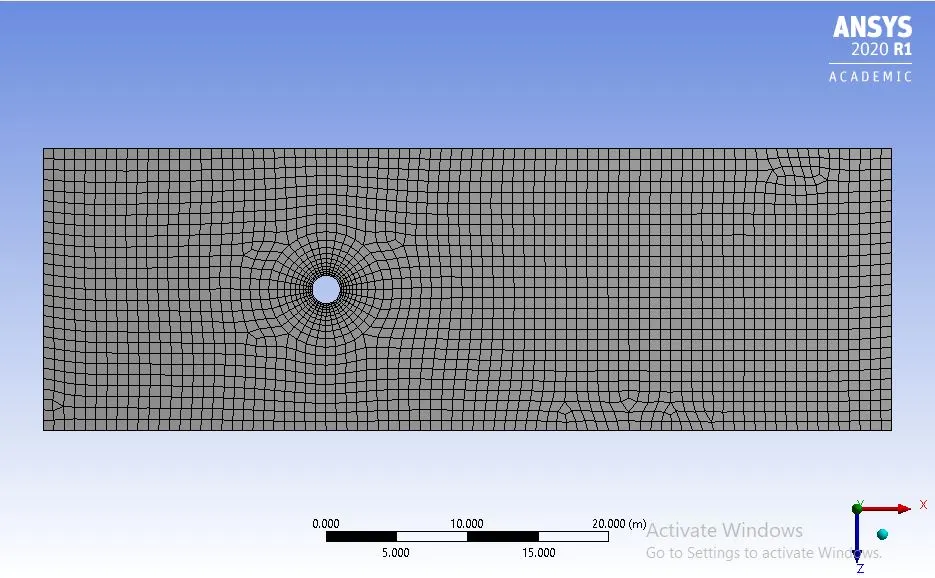
Fig. 2: Mesh 1 for Reynolds number 10 with 10 inflation layers

Mesh 2 for Reynolds number 10:

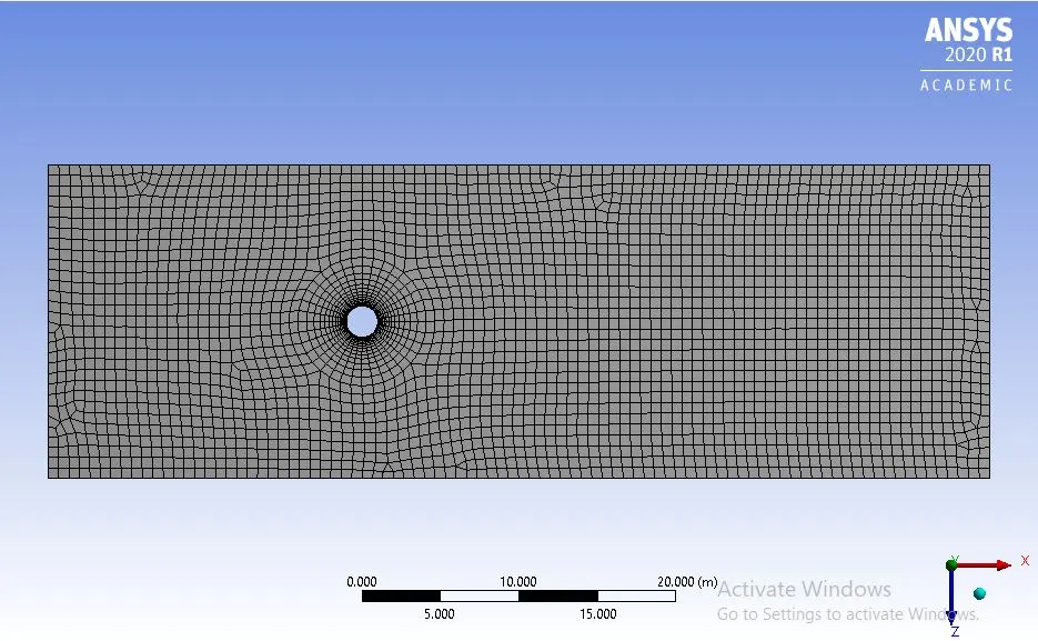
Fig. 3: Mesh 2 for Reynolds number 10 with 15 inflation layers

Mesh 3 for Reynolds number 10:

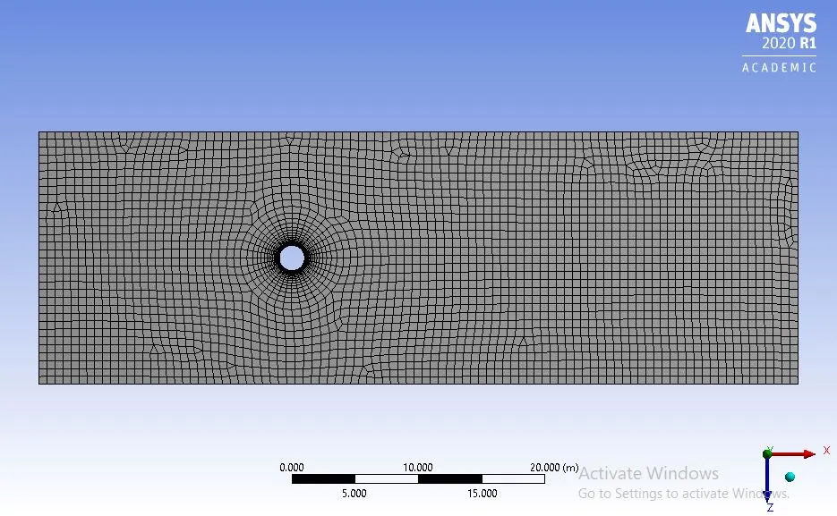
Fig. 4: Mesh 3 for Reynolds number 10 with 20 inflation layers

Mesh 4 for Reynolds number 10:

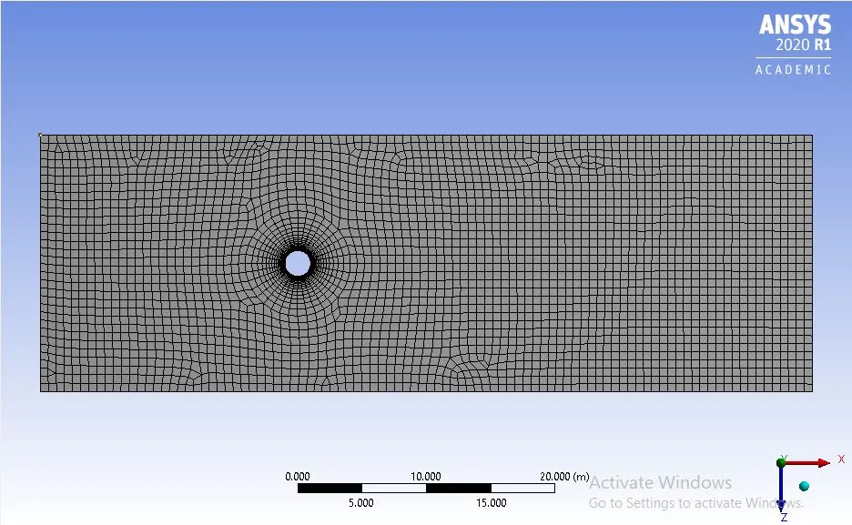
Fig. 5: Mesh 4 for Reynolds number 10 with 25 inflation layers

For Reynolds number 10:

Mesh	Element-Size(m)	Nodes	Elements	No. of Inflation Layers	Coefficient of Drag(Cd)	%var
1	0.7402	2573	2448	10	3.3076	--
2	0.6637	3221	3086	15	3.3268	+0.58
3	0.6304	3662	3523	20	3.3332	+0.19
4	0.6275	3893	3749	25	3.3360	+0.08

Table 8: Mesh statistics, no. of inflation layers, coefficient of drag values and percentage variation for Reynolds number 10

Mesh quality attributes for Reynolds number 10:

Mesh	Element Quality(avg.)	Aspect Ratio(avg.)	Skewness(avg.)	Orthogonal Quality(avg.)
1	0.95787	Quadrilaterals-1.0756	0.046655	0.99464
2	0.92088	Quadrilaterals-1.2508	0.055141	0.9941
3	0.88208	Quadrilaterals-1.6163	0.05666	0.99311
4	0.84369	Quadrilaterals-2.5024	0.055485	0.99319

Table 9: Mesh quality attributes depicting the average values of element quality, aspect ratio, skewness and orthogonal quality for four different mesh element sizes for Reynolds number 10

Similar to Reynolds number 10 and using the values of laminar boundary layer thickness in Table 6 with a starting number of 10 inflation layers, a mesh independence study for Reynolds number 100 was performed which had the following impacts:

Mesh	No. of Inflation Layers	Initial Height (m) (Eq. 7)	Element Size (m) (Eq. 8)
1	10	0.03783	0.234
2	15	0.0136	0.21
3	20	0.00526	0.2016
4	25	0.00208	0.198
5	30	0.000831	0.1974

Table 10: Element Size (m) determination using number of inflation layers and calculation of initial height from Laminar boundary thickness value for Reynolds number 100

Mesh 1 for Reynolds number 100:

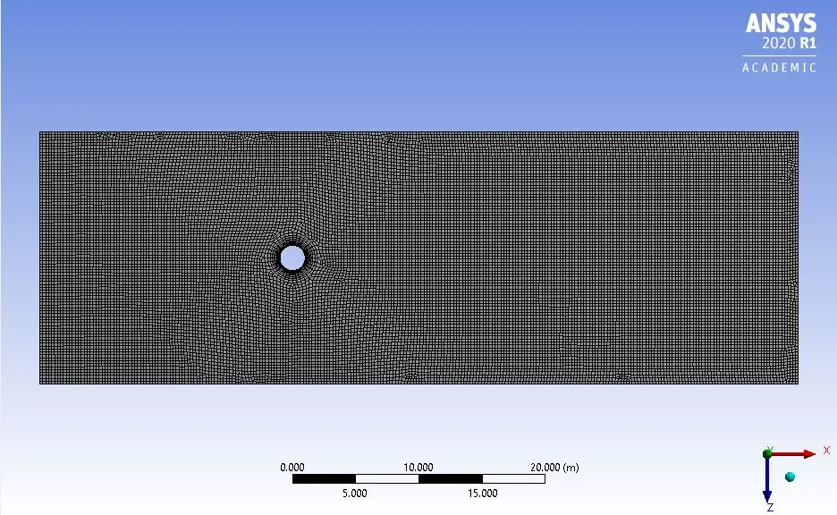
Fig. 6: Mesh 2 for Reynolds number 100 with inflation layers 10

Mesh 2 for Reynolds number 100:

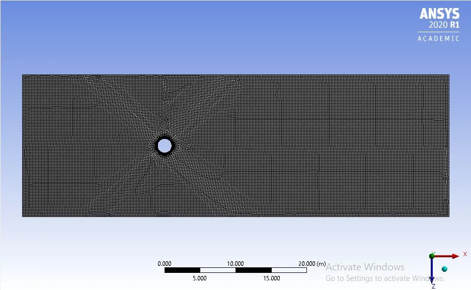
Fig. 7: Mesh 2 for Reynolds number 100 with inflation layers 15

Mesh 3 for Reynolds number 100:

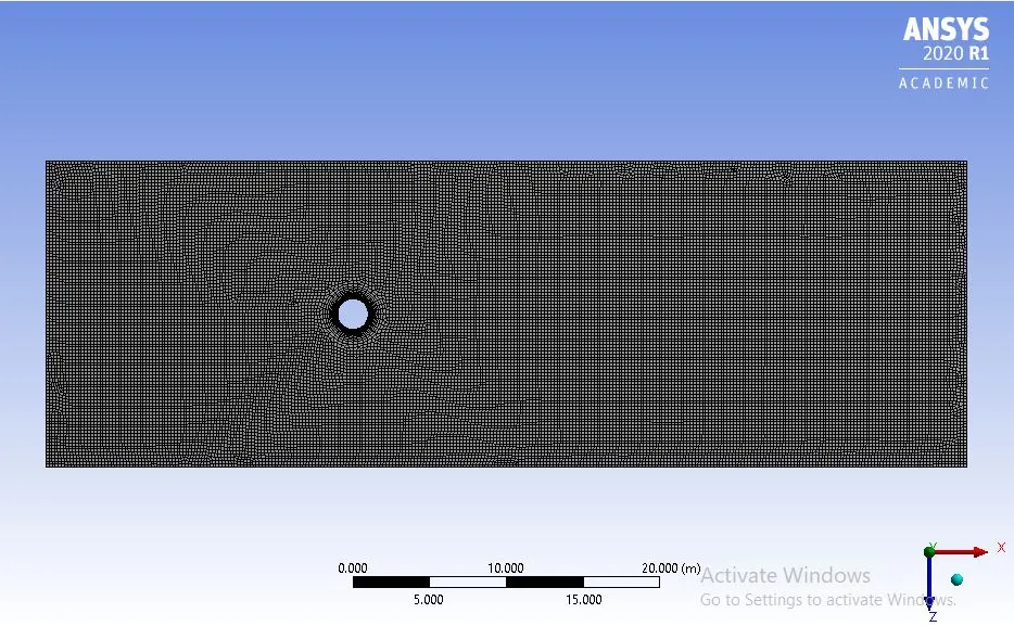
Fig. 8: Mesh 3 for Reynolds number 100 with inflation layers 20

Mesh 4 for Reynolds number 100:

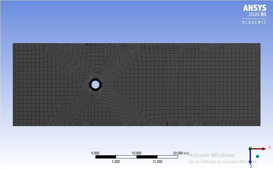
Fig. 9: Mesh 4 for Reynolds number 100 with inflation layers 25

Mesh 5 for Reynolds number 100:

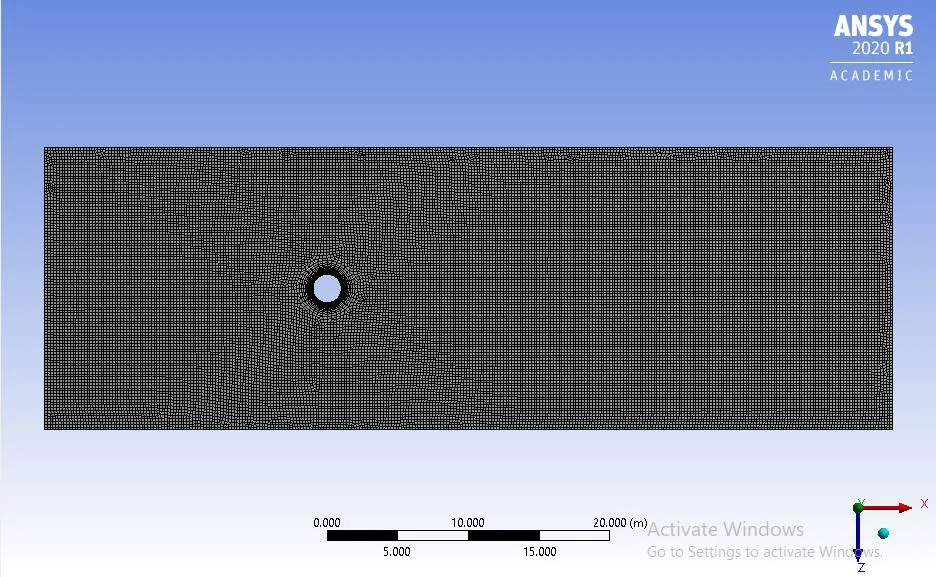
Fig. 10: Mesh 5 for Reynolds number 100 with inflation layers 30

For Reynolds number 100:

Mesh	Element-Size(m)	Nodes	Elements	No. of Inflation Layers	Coefficient of Drag(Cd)	%var
1	0.234	21928	21574	10	1.3704	--
2	0.21	27355	26960	15	1.3662	-0.31
3	0.2016	30129	29722	20	1.3751	+0.65
4	0.198	31197	30780	25	1.3721	-0.22
5	0.1974	31761	31344	30	1.3615	+0.77

Table 11: Mesh statistics, no. of inflation layers, coefficient of drag values and percentage variation for Reynolds number 100

Mesh quality attributes for Reynolds number 100:

Mesh	Element Quality(avg.)	Aspect Ratio(avg.)	Skewness(avg.)	Orthogonal Quality(avg.)
1	0.9686	Quadrilaterals-1.0613	0.030232	0.99619
2	0.96837	Quadrilaterals-1.1121	0.025204	0.99739
3	0.96463	Quadrilaterals-1.2573	0.0237	0.99771
4	0.96009	Quadrilaterals-1.6041	0.023073	0.99747
5	0.95443	Quadrilaterals-2.4702	0.023727	0.99755

Table 12: Mesh quality attributes depicting the average values of element quality, aspect ratio, skewness and orthogonal quality for five different mesh element sizes for Reynolds number 100

From the above meshing statistics with regards to the number of inflation layers, mesh number 3 (or mesh 3) for Reynolds number 10 with element size 0.6304m and 20 inflation layers represents a mesh independent result in terms of minimum percentage variation (%var) of the coefficient of drag values especially when compared with mesh 4 as the difference in values is quite small i.e., to the order of 1e-02. In the case of Reynolds number 100, it is observed from Table 11 that the trend for variation in coefficient of drag values is less than 1% and that both mesh 3 and mesh 4 record the least difference in values for the same. As a result, choosing either of the two meshes would not lead to a huge difference and therefore, for this simulation it was decided to choose mesh 4 with element size of 0.198m and number of inflation layers as 25 to be the mesh independent solution. The %var is calculated as the ratio of the difference of the coefficient of drag values in two consecutive meshes to the coefficient of drag value of the previous mesh e.g., ((Coefficient of drag for Mesh 2 - Coefficient of drag for Mesh 1)/Coefficient of drag for Mesh 1). Also, the quality attributes of all four meshes for Reynolds number 10 and five meshes for Reynolds number 100 mentioned in Table 9 and Table 12 respectively with varying element sizes indicates that they all lie in the range of 'good' to 'excellent' scale. Results for Reynolds number 10 and Reynolds number 100 will only be referred with regards to their mesh independent solutions in the rest of the report.

Section 2.5.2 Mesh Refinement approach for Flow Regime of Laminar to Turbulent Transition in Wake

Similar to the strategy adopted for mesh creation for Reynolds number 10 and 100 and retaining the mesh quality attributes outlined in Section 2.2 Meshing, a quadrilateral dominant mesh type was selected for the entire domain with near wall refinement performed using 'Edge Sizing' and 'Number of Divisions' set to 36. In order to add inflation layers to capture the flow accurately around the cylinder with regards to predicting coefficient of drag (Cd) and coefficient of lift (Cl) values, the boundary layer development for flow around the cylinder was required to be calculated based on the transition of flow properties from laminar to turbulent which is shown below:

Predicting near wall cell-size for Reynolds number 1000, 10000 and 100000:

Since, the flow around circular cylinder for Reynolds number 1000, 10000 and 100000 as found out from experimental findings of Roshko (1954) [5] lies in the flow regime of laminar to turbulent transition region and that the wake demonstrates an “irregular” regime wherein the velocity fluctuations represent clear irregularities although the boundary layer separation continues to be laminar as was also confirmed by Sumer (1997) [6]. Therefore, (Eq. 5) can be reused to calculate the Laminar boundary thickness.

For Reynolds number 1000, 10000 and 100000 with dynamic viscosity value of 0.05 `(kg)/(ms)`, density value of 1 `(kg)/m^3` and free-stream velocity values from input boundary conditions in Table 2, the laminar boundary layer thickness using Eq. 2 are calculated in the following table:

Reynolds Number	Freestream velocity (U) (m/s)	Laminar boundary layer Thickness (m) (Eq. 2)
1000	25	0.3105
10000	250	0.0982
100000	2500	0.0031

Table 13: Freestream velocity and Laminar boundary layer thickness values for Reynolds number 1000, 10000 and 100000

However, since the flow belongs to an “irregular” regime, also called as the Shear-Layer Transition Regime, the instability in the wake formation is as a result of the separating shear layers from either side of the circular cylinder thereby implying the transition towards a more turbulent behaviour. In order to capture this wake formation behaviour near the wall and to understand the impact of drag and lift forces on the wall, we need to make use of a turbulence model that resolves the viscous sub layer for which the first grid cell, in this case at the first cell height, needs to be at a value of y+ equal to 1. To ensure y+ value of 1, we need to calculate the values of wall shear stress and frictional velocity as shown below:

For Wall Shear Stress:

`tau_w = (1/2)*C_f*rho*(U_(infty))^(2)`, where (Eq. 9)

`tau_w` is Wall shear stress,

`C_f` is Skin Friction coefficient,

`rho` is Density of fluid, and

`U_infty` is the freestream velocity which is calculated from the Reynolds number formula mathematically as `(Re*mu)/(D*rho)`

Skin Friction Coefficient (`C_f`), also according to Blasius, for external flows can be related to the Reynolds number as shown below:

`C_f = 0.664/(sqrt (Re_x))`, where (Eq. 10)

`Re_x` represents Reynolds number at a distance 'x' from the leading edge in the direction of flow

Frictional velocity (`U_tau`) can be computed mathematically as:

`U_tau = sqrt ((tau_w)/(rho))` (Eq. 11)

`y^(+)` is defined as the non-dimensional wall distance for a wall bounded flow that can be expressed mathematically as:

`y^+=(ρ*U_tau*y_P)/mu`; where (Eq. 12)

`y_P` is distance from the cell-centroid 'P' to the wall such that `Delta_y = 2*y_P`. In other words, `y^(+)` at `y_P` is ensured to be 0.5, which is well within the demarcated boundaries for viscous sub-layer, such that a corresponding `y^(+)` at `Delta_y` would be equal to 1.

Simplifying (Eq. 12) to determine First Cell Height (`Delta_y`), we get;

`Delta_y = 2*(y^(+)*mu)/(rho*U_tau)` (Eq. 13)

For Reynolds number 1000, 10000 and 100000 with dynamic viscosity value of 0.05 `(kg)/(ms)`, density value of 1 `(kg)/m^3`, free-stream velocity values from input boundary conditions in Table 2 and `y^(+)` value of 1, the skin-friction coefficient (`C_f`), wall shear stress (`tau_w`), friction velocity (`U_tau`) and eventually the first cell height (`Delta_y`) values using (Eq. 10), (Eq. 9), (Eq. 11) and (Eq. 13) respectively are calculated in the following table:

Reynolds Number	Skin-friction Coefficient (`C_f`)	Wall Shear Stress (`tau_w`)[kg m^-1 s^-2]	Friction Velocity (`U_tau`) [m s^-1]	First Cell Height (`Delta_y`) [m]
1000	0.021	6.5625	2.5617	0.01952
10000	0.00664	207.5	14.405	0.003471
100000	0.0021	6562.5	81.009	0.00061721

Table 14: Skin-friction coefficient, wall shear stress, friction velocity and first cell height values for Reynolds number 1000, 10000 and 100000

Calculation of Inflation Layers based on First Cell Height (`Delta_y`) and Laminar Boundary Layer Thickness (`delta_L`):

As previously mentioned, the default growth rate type for determining height of inflation layers is Geometric and the total height at layer 'n' for geometric growth rate type is defined in (Eq. 6). However, in this case, the initial height (h) is known which is equal to the value of the first cell height (`Delta_y`). Therefore, the missing variable in (Eq. 6) is n or in this case, total number of inflation layers. Also, element size can be determined from (Eq. 8). The values computed for total number of inflation layers from (Eq. 6) and element size from (Eq. 8) is tabulated below:

Reynolds Number	No. of Inflation Layers (Eq. 6)	Element Size (m) (Eq. 8)	Height ratio (r) (Eq. 8)
1000	8	0.0955	1.2
10000	11	0.08995	1.25
100000	14	0.07225	1.3

Table 15: Number of inflation layers and Element Size (m) determination using first cell height (`Delta_y`) as initial height and Laminar boundary thickness value for Reynolds number 1000, 10000 and 100000

The use of different height ratio values in (Eq.8) to compute element size values was due to constraints in computational resources and limitations in maximum number of cells/nodes for solution by ANSYS Student license to 512,000. These challenges also restricted from performing mesh independence study based on the given `y^(+)` value to work with element sizes smaller than those shown in Table 15 corresponding to their respective Reynolds number.

Mesh for Reynolds number 1000:

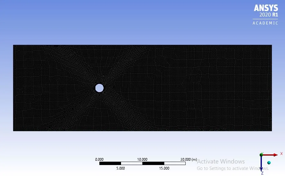
Fig. 11: Mesh for Reynolds number 1000 with first cell height (`Delta_y`) at 0.01952m and inflation layers 8

Mesh for Reynolds number 10000:

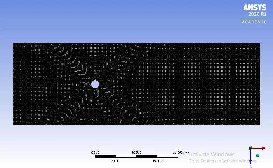
Fig. 12: Mesh for Reynolds number 10000 with first cell height (`Delta_y`) at 0.003471m and inflation layers 11

Mesh for Reynolds number 100000:

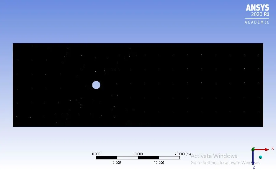
Fig. 13: Mesh for Reynolds number 100000 with first cell height (`Delta_y`) at 0.00061721m and inflation layers 14

Mesh statistics, no. of inflation layers and coefficient of drag values for Reynolds number 1000, 10000 and 100000:

Reynolds Number	Element-Size(m)	Nodes	Elements	No. of Inflation Layers	Coefficient of Drag(Cd)
1000	0.0955	130022	129159	8	1.4018
10000	0.08995	147448	146531	11	1.4047
100000	0.07225	229783	228637	14	0.8354

Table 16: Mesh statistics, no. of inflation layers and coefficient of drag values for Reynolds number 1000, 10000 and 100000

Mesh quality attributes for Reynolds number 1000, 10000 and 100000:

Reynolds Number	Element Quality(avg.)	Aspect Ratio(avg.)	Skewness(avg.)	Orthogonal Quality(avg.)
1000	0.98535	Quadrilaterals-1.0224	0.015158	0.99862
10000	0.98381	Quadrilaterals-1.0832	0.013767	0.99894
100000	0.98782	Quadrilaterals-1.2971	0.0081752	0.99954

Table 17: Mesh quality attributes depicting the average values of element quality, aspect ratio, skewness and orthogonal quality for Reynolds number 1000, 10000 and 100000

2.5.3 Convergence Level

In the given numerical analysis, we are performing both a steady-steady and transient simulation using a Pressure based solver of type SIMPLE scheme which is iterative in nature, computationally quicker than other pressure-based solvers while also allowing more iterations to be performed in the same time and with respect to the current problem, the changes in consecutive solutions i.e., velocity and pressure values are no longer small with increasing Reynolds number. The selection of schemes for the different terms under spatial discretization includes assigning Gradient to Least Squares Cell Based scheme, pressure to second order scheme, momentum to second order upwind scheme, Turbulent Kinetic Energy to first order upwind scheme and Turbulent Dissipation Rate to first order upwind scheme of which the Turbulent Kinetic Energy and Turbulent Dissipation Rate is applicable only for the k-`omega` SST turbulence model. Least Squares Cell Based scheme is the default gradient method chosen by ANSYS Fluent which is used to compute the change in values across the centroid of two cells along a vector path and is a computationally less expensive scheme offering comparable accuracy to the node-based gradient scheme, both of which are superior to the cell-based gradient scheme. The second order scheme for the pressure makes use of the central differencing scheme and is generally considered to be more accurate than the Standard and Linear schemes as well as robust in the case of skewed meshes. A second order upwind scheme is chosen for the momentum and energy terms that makes use of the quantities at the cell face values to compute a cell-centered solution at the cell centroid leading to a second order accurate solution. The turbulence terms viz., Turbulent Kinetic Energy and Turbulent Dissipation Rate are set at first order upwind scheme by default which makes use of quantities at the cell faces as the cell-average value indicating that it is first-order accurate. The reason to have the turbulence terms discretized using the first-order upwind scheme is based on observations from simulations across different applications when using a higher or even second order upwind scheme leads the computational cost to become more expensive (more compute time) solution while also demonstrating stability issues in the form of repeating oscillations of values and not necessarily guaranteeing always a more accurate solution. For both the steady-state and transient solutions for the given flow field, the convergence criteria option has been checked off, however, the residual values which measures the local imbalance of conserved variable in each control volume, in this case the turbulence model equations such as continuity, x-velocity, y-velocity, k and `omega` are being monitored throughout the solution process for the defined number of iterations so as to not restrict the development of the actual fluid behaviour, as part of the physical process, during the formation of the Karman vortex street and laminar to turbulent wake transition. Also, as previously mentioned in Section 2.3.3 Boundary Conditions and Monitoring Points, we are monitoring the behaviour of velocity at the monitor point using the 'vertex-average' option from the 'Surface Report' list as the quantity of interest to observe the variation in values over successive iterations. The residual limits defined for the equations corresponding to the laminar and turbulence model equations and the residual plots corresponding to the different meshes and different input conditions are shown in the table and figures below:

	laminar	k-`omega` SST
continuity	1e-03	1e-03
x-velocity	1e-03	1e-03
y-velocity	1e-03	1e-03
k	--	1e-03
omega	--	1e-03

Table 18: Residual Values of the different equations used in the laminar and k-`omega` SST turbulence model

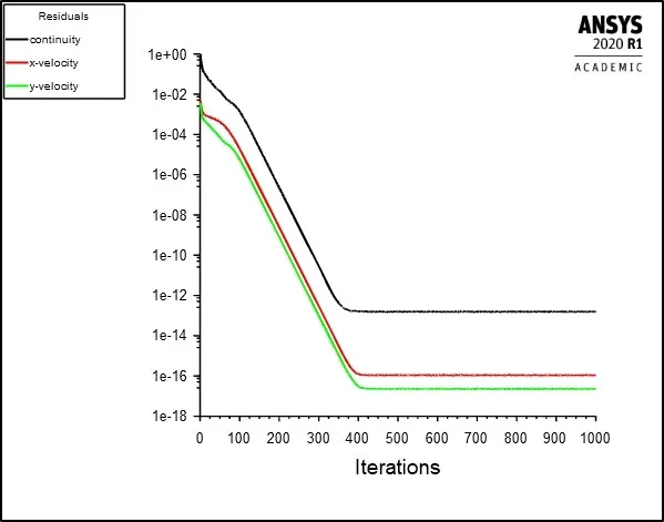
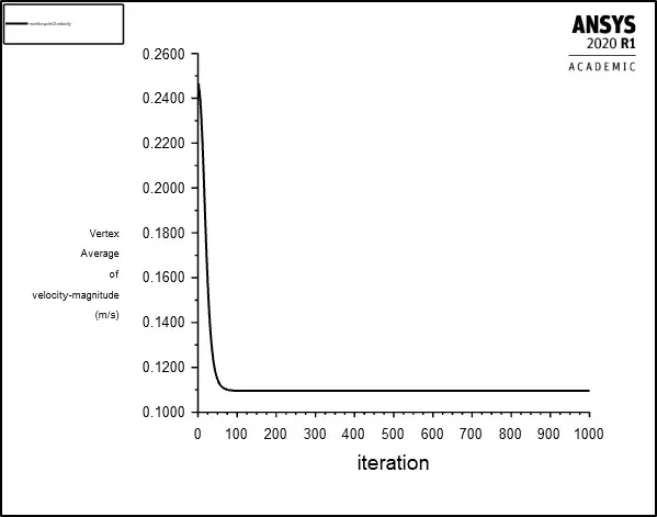
Fig. 14: Residuals Plot and Vertex Average of Velocity Magnitude (m/s) at the monitor point for steady-state simulation using laminar model for mesh 1 of Reynolds number 10

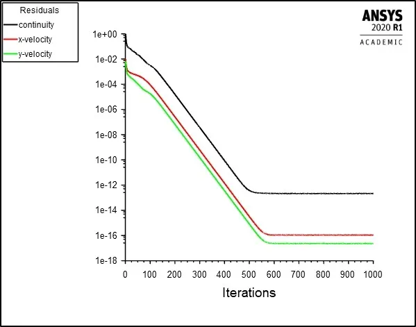
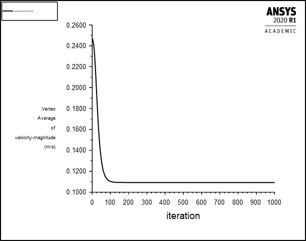Fig. 15: Residuals Plot and Vertex Average of Velocity Magnitude (m/s) at the monitor point for steady-state simulation using laminar model for mesh 2 of Reynolds number 10

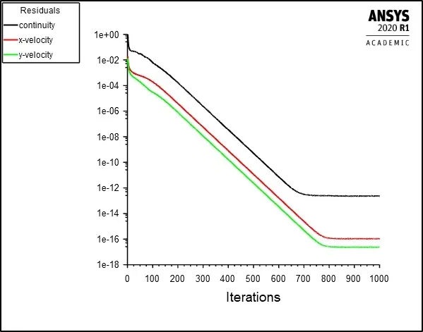
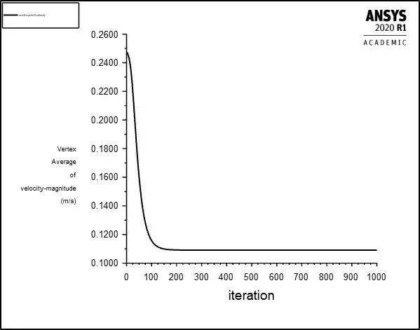
Fig. 16: Residuals Plot and Vertex Average of Velocity Magnitude (m/s) at the monitor point for steady-state simulation using laminar model for mesh 3 of Reynolds number 10

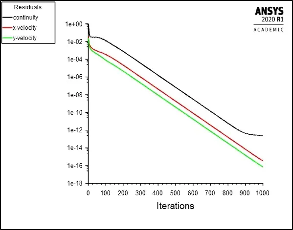
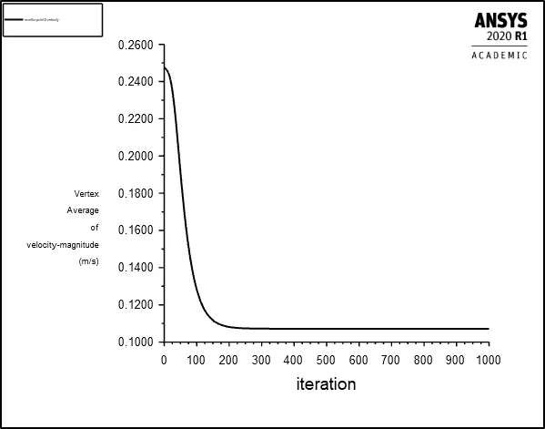Fig. 17: Residuals Plot and Vertex Average of Velocity Magnitude (m/s) at the monitor point for steady-state simulation using laminar model for mesh 4 of Reynolds number 10

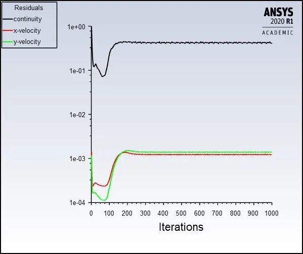
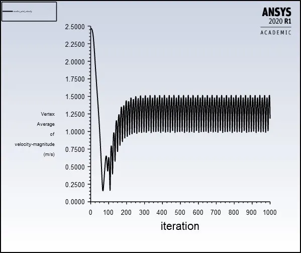Fig. 18: Residuals Plot and Vertex Average of Velocity Magnitude (m/s) at the monitor point for steady-state simulation using laminar model for mesh 1 of Reynolds number 100

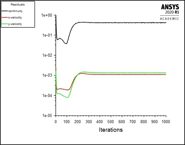
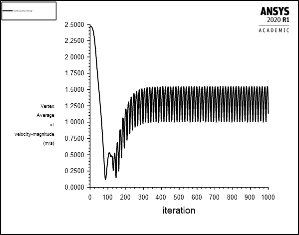Fig. 19: Residuals Plot and Vertex Average of Velocity Magnitude (m/s) at the monitor point for steady-state simulation using laminar model for mesh 2 of Reynolds number 100

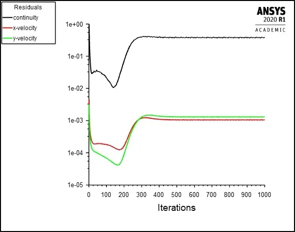
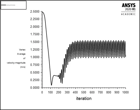Fig. 20: Residuals Plot and Vertex Average of Velocity Magnitude (m/s) at the monitor point for steady-state simulation using laminar model for mesh 3 of Reynolds number 100

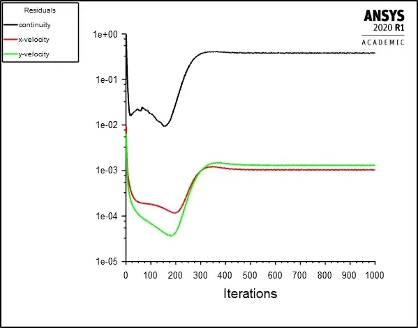
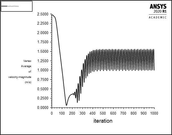Fig. 21: Residuals Plot and Vertex Average of Velocity Magnitude (m/s) at the monitor point for steady-state simulation using laminar model for mesh 4 of Reynolds number 100

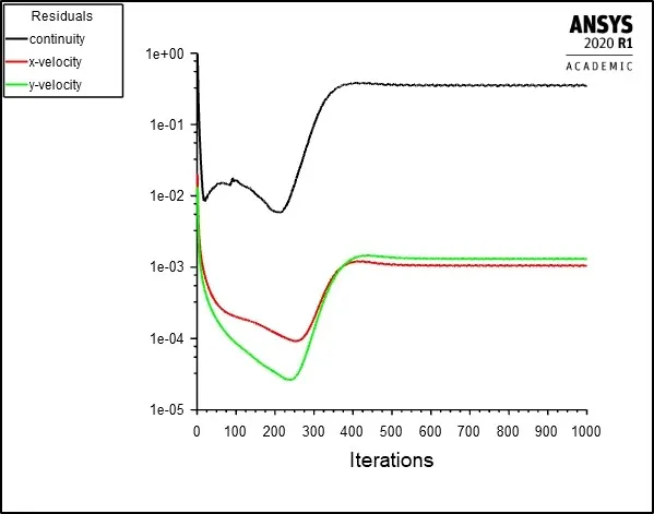
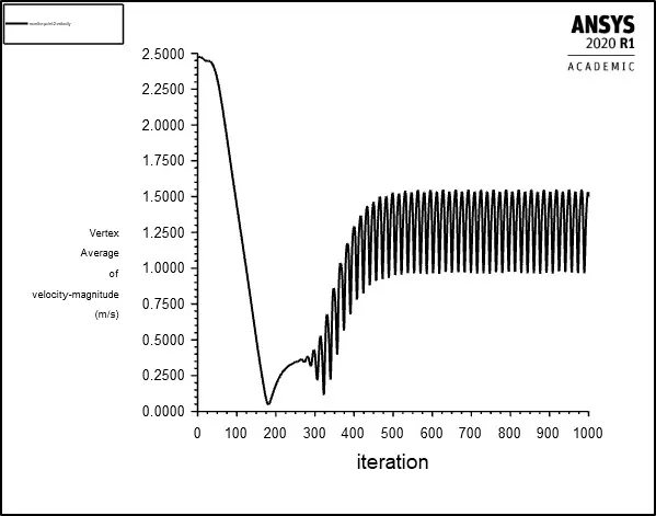Fig. 22: Residuals Plot and Vertex Average of Velocity Magnitude (m/s) at the monitor point for steady-state simulation using laminar model for mesh 5 of Reynolds number 100

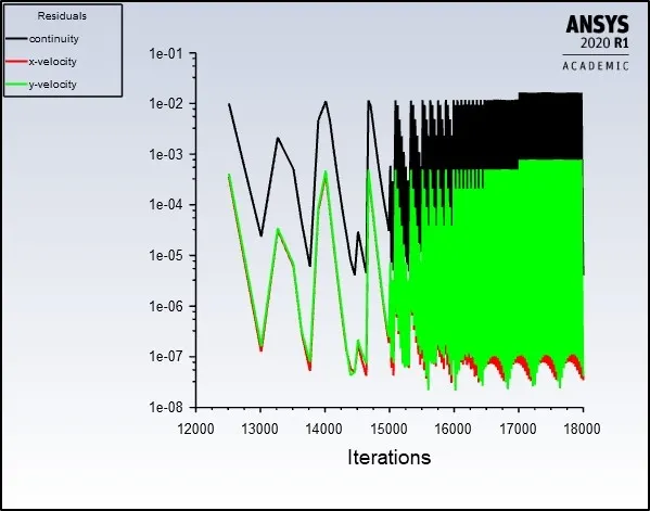
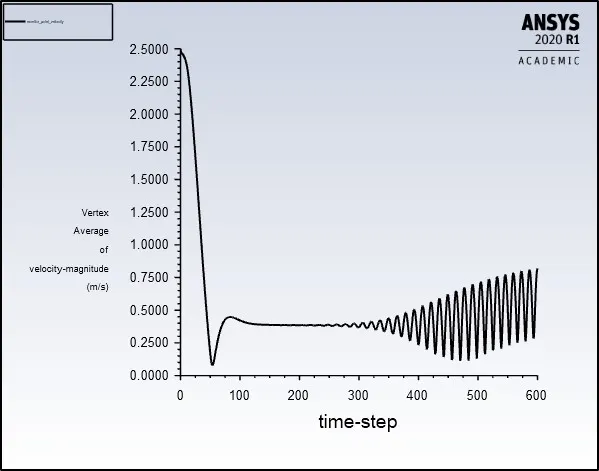Fig. 23: Residuals Plot and Vertex Average of Velocity Magnitude (m/s) at the monitor point for unsteady-state simulation using laminar model for mesh 4 of Reynolds number 100

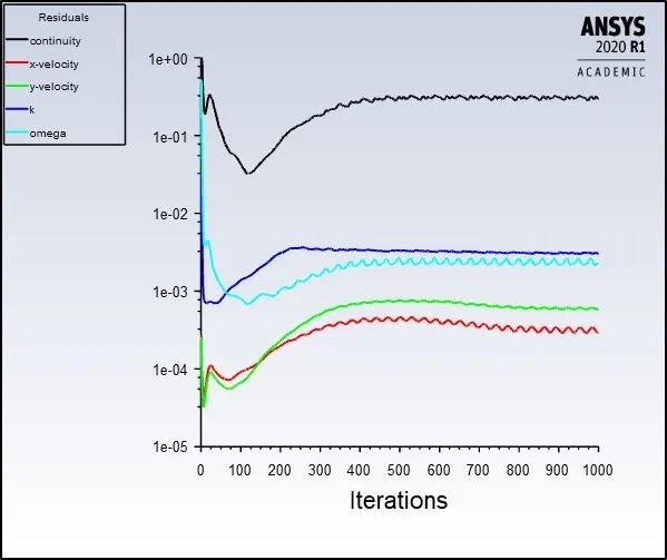
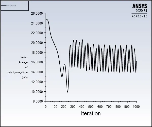Fig. 24: Residuals Plot and Vertex Average of Velocity Magnitude (m/s) at the monitor point for steady-state simulation using k-`omega` SST turbulence model for mesh of Reynolds number 1000

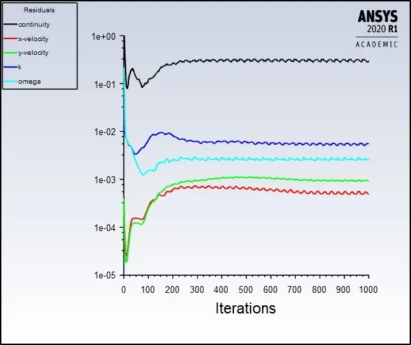
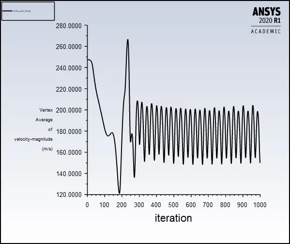Fig. 25: Residuals Plot and Vertex Average of Velocity Magnitude (m/s) at the monitor point for steady-state simulation using k-`omega` SST turbulence model for mesh of Reynolds number 10000

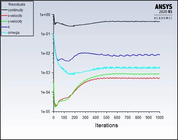
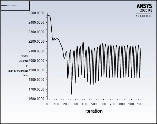
Fig. 26: Residuals Plot and Vertex Average of Velocity Magnitude (m/s) at the monitor point for steady-state simulation using k-`omega` SST turbulence model for mesh of Reynolds number 100000

From Fig. 14, Fig. 15, Fig. 16 and Fig. 17, we can notice that for Reynolds number 10, the residuals have converged based on the residual values mentioned in Table 18 and Vertex Average plot of Velocity Magnitude (m/s) at the monitor point shows a highly stable output well before they reach the total number of iterations indicating that a steady-state solution has been obtained. However, Fig. 18, Fig. 19, Fig. 20, Fig. 21, Fig. 22, Fig. 24, Fig. 25 and Fig. 26, demonstrates the residuals to have a gradual decline first followed by gradual rise before becoming stable and when compared with the Vertex Average plot of Velocity Magnitude (m/s) at the monitor point shows an oscillating behaviour in the velocity values. This recurrence of oscillating velocity values, especially for Reynolds number 100, indicates that the solution is time-dependent as the phenomena of Karman vortex street beyond Reynolds number 40, observed from experimental findings, takes dominance in the wake formation beyond the circular cylinder in the direction of flow. To confirm the time-dependent behaviour of the velocity values it can be seen in Fig. 23 for Reynolds number 100 that the Vertex Average plot of Velocity Magnitude (m/s) at the monitor point has a stable output somewhere close to 200 iterations after which the values begin to oscillate, at first with irregular intervals before becoming evenly spaced out with an almost constant frequency value. This variation is characteristic of the wake formation behaviour with regards to the Karman vortex street phenomena since it develops slowly over time on the surface of the circular cylinder before becoming consistent. It is important to note that the residual values remain unaltered as seen in Table 18 for the transient state simulation and that for each time step the solution variables are converged with regards to the maximum iterations set for each time step.

3. Results

In reference to Fig. 1, Coefficient of drag and lift on the cylinder wall, Vortex shedding behind the cylinder using velocity and static pressure, and streamline plots have been created that would signify the development of lift and drag forces as well as demonstrate the development of velocity and static pressure profiles for the different fluid conditions for mesh independent solutions for Reynolds number 10 and 100 and mesh refined based on `y^(+)` values for Reynolds number 1000, 10000 and 100000.

3.1 Coefficient of drag and lift on the cylinder wall, Vortex shedding behind the cylinder using velocity, and static pressure and streamline plots

The figures below i.e., Fig. 27, Fig. 28 and Fig. 29, shows the Coefficient of drag and lift on the cylinder wall, Vortex shedding behind the cylinder using velocity, and static pressure and streamline plots for Reynolds number 10. It can be seen from Fig. 27 that the coefficient of drag and lift values have steady state solutions well before the total number of iterations has been reached which can be attributed to the presence of a steady wake region beyond the cylinder as seen in Fig. 28 and Fig. 29 (streamline plot). The static pressure contour plot illustrates the regions of high pressure which is generally characterised in the vicinity of the cylinder wall where the velocity values are low while low pressure regions are observed away from the cylinder where the velocity, because of the laminar velocity profile, comes closer to the free-stream velocity value. However, for Reynolds number 100 and above, the wake no longer remains steady and the phenomena of Karman vortex street assumes dominance. In the case of Reynolds number 100, the coefficient of drag has a stable output while the coefficient of lift has a recurring oscillatory behaviour. This is because the wake is no longer stable implying that the strength and amplification of the vortices have increased significantly as can be seen by the highly varying vortex structures in Fig. 31 and Fig. 32 (streamline plot). Since, the frequency at which the vortices are being generated have an almost consistent value, a transient state simulation further confirms the time-dependence behaviour of vortex shedding as can be seen in Fig. 42, Fig. 44 and Fig. 45 with peak Strouhal number at 0.150 in Fig. 43 validating well against the experimental value reported by Tritton (1959) [3] of 0.164. In the case of Reynolds number 1000, 10000 and 100000, the variation in pressure values from the lowest pressure point to the increase in surface pressure values in the downstream direction is almost exponential as can be seen in Fig. 35, Fig. 38 and Fig. 41 (static pressure contour plot). This is because the vortex shedding process is no longer laminar as was observed with Reynolds number 100 and the instabilities in the wake are also contributed by the rise in three-dimensional distortions especially due to the separating shear layers from the sides of the cylinder and eventually leading to turbulent behaviour. Therefore, the coefficient of drag and lift plots in Fig. 33, Fig. 36 and Fig. 39 have an oscillating plot of unequal peak amplitude values.

Steady state:

For Reynolds number 10:

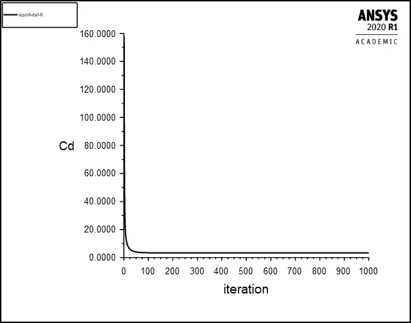
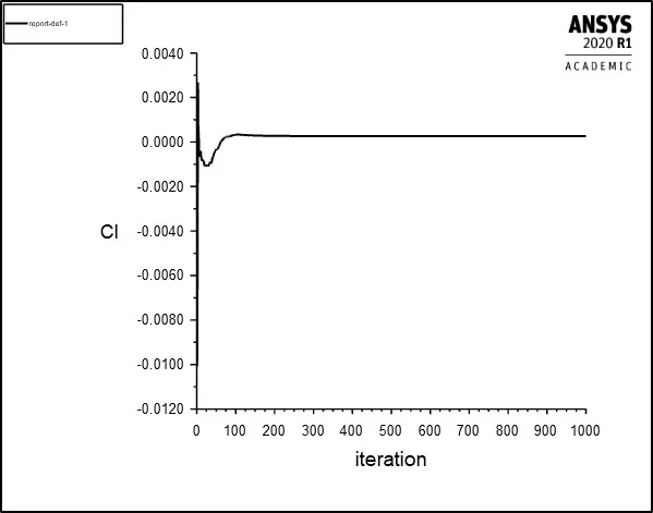Fig. 27: Coefficient of drag and lift on the cylinder wall for Reynolds number 10

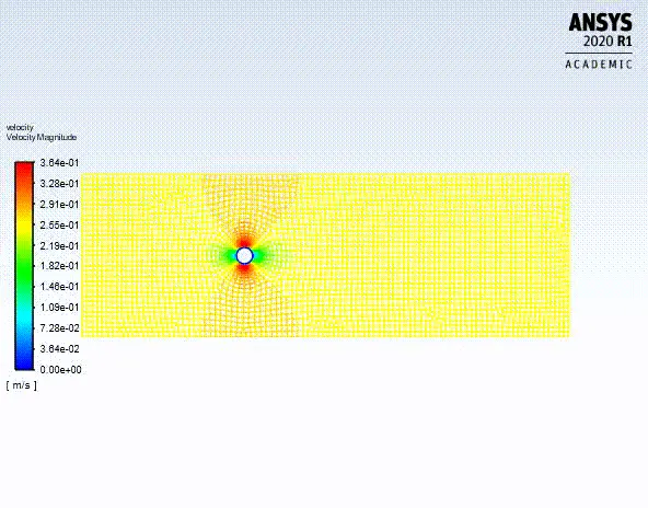
Fig. 28: Velocity contour animation plot for Reynolds number 10

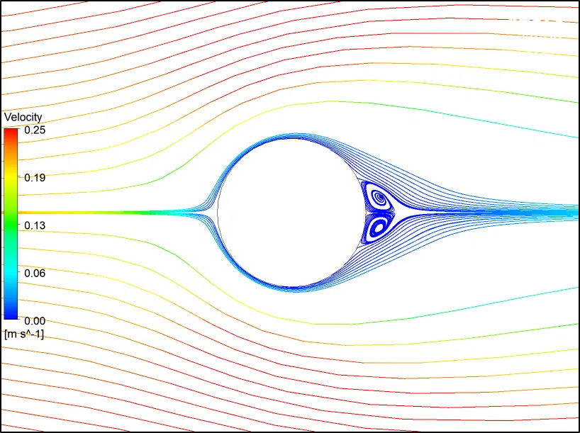
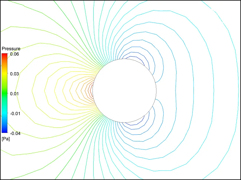Fig. 29: Streamline and static pressure contour (showing contour lines only) plots for Reynolds number 10

For Reynolds number 100:

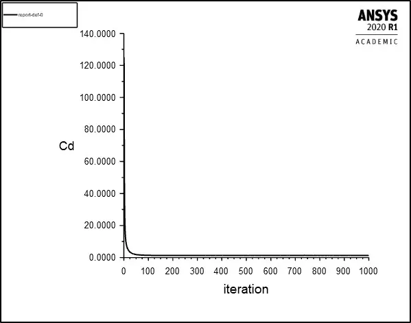
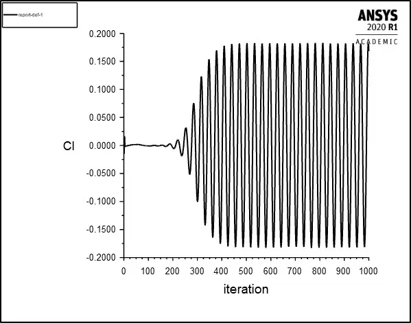Fig. 30: Coefficient of drag and lift on the cylinder wall for Reynolds number 100

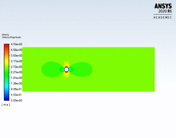
Fig. 31: Vortex shedding behind the cylinder using velocity contour animation plot for Reynolds number 100

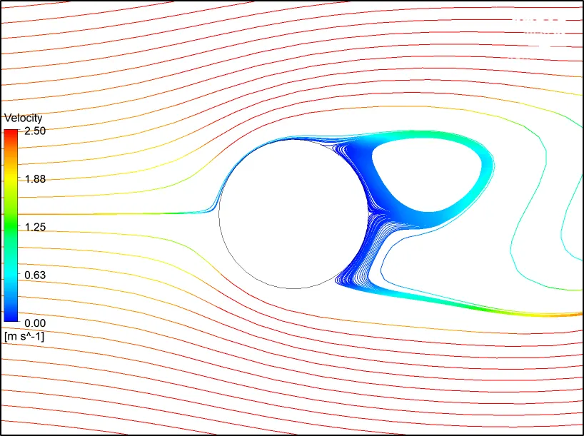
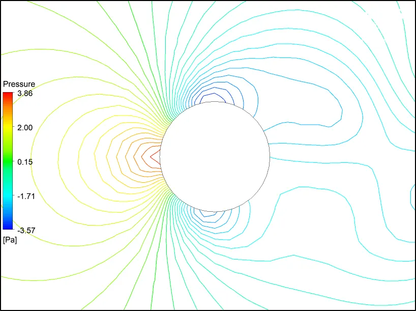Fig. 32: Streamline and static pressure contour (showing contour lines only) plots for Reynolds number 100

For Reynolds number 1000:

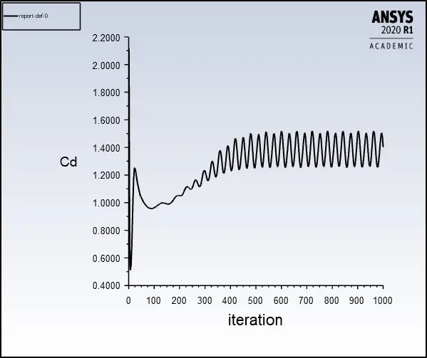
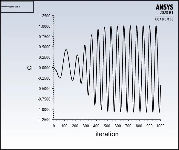Fig. 33: Coefficient of drag and lift on the cylinder wall for Reynolds number 1000

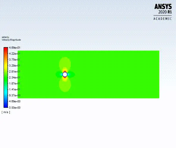
Fig. 34: Vortex shedding behind the cylinder using velocity contour animation plot for Reynolds number 1000

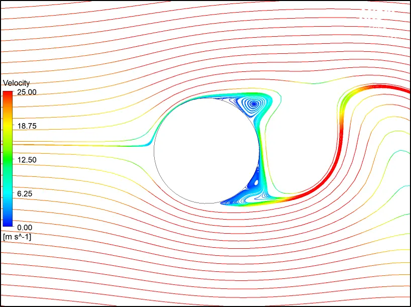
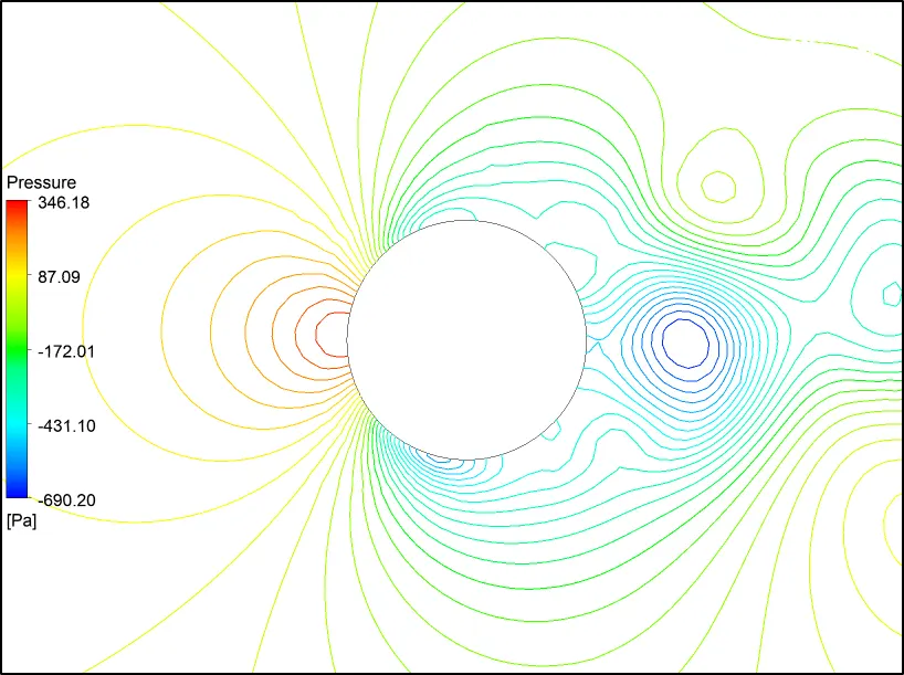Fig. 35: Streamline and static pressure contour (showing contour lines only) plots for Reynolds number 1000

For Reynolds number 10000:

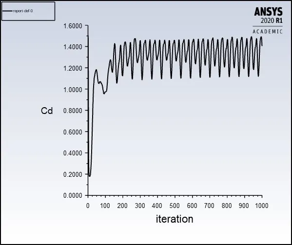
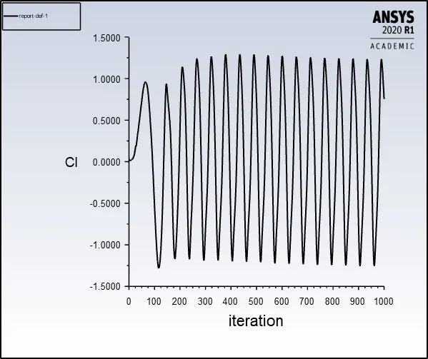Fig. 36: Coefficient of drag and lift on the cylinder wall for Reynolds number 10000

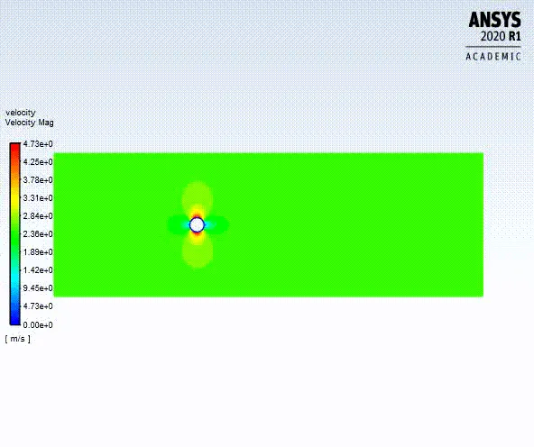
Fig. 37: Vortex shedding behind the cylinder using velocity contour animation plot for Reynolds number 10000

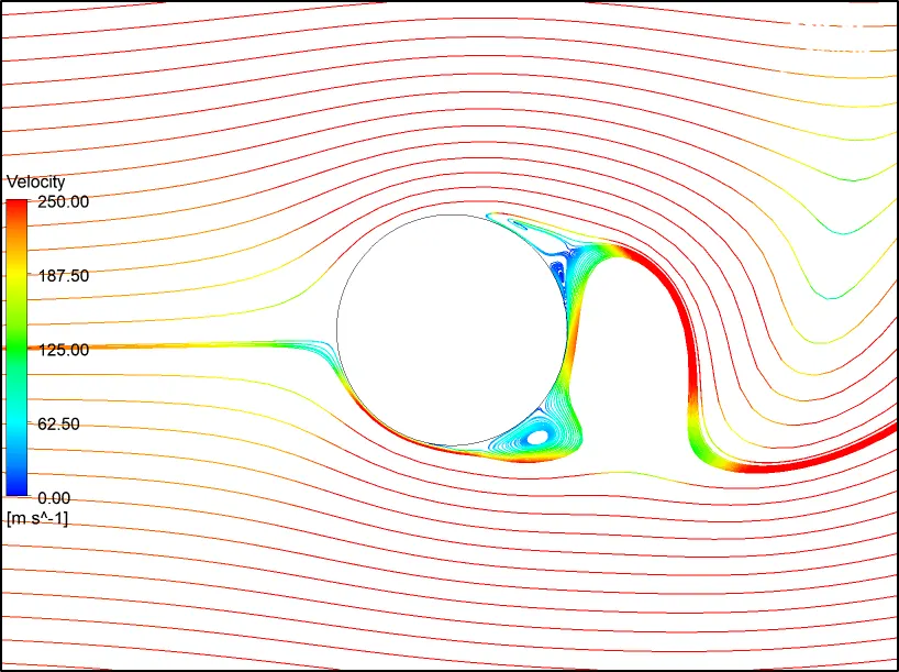
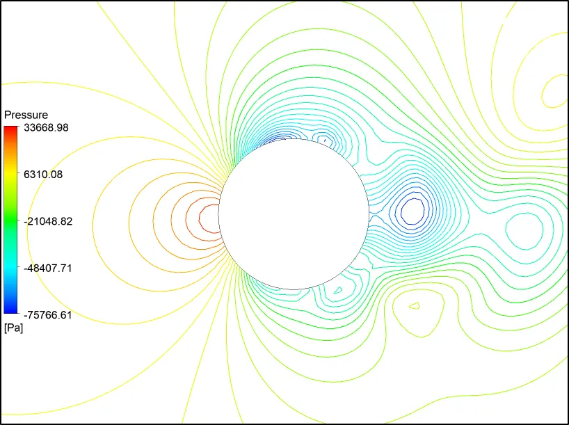Fig. 38: Streamline and static pressure contour (showing contour lines only) plots for Reynolds number 10000

For Reynolds number 100000:

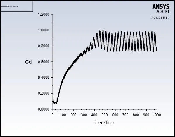
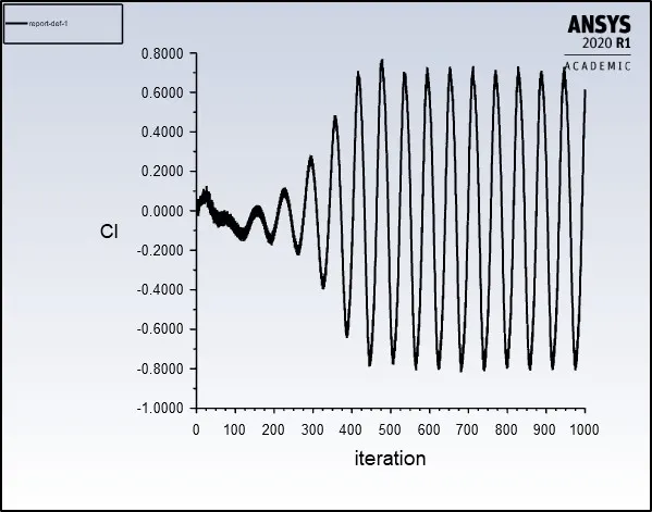Fig. 39: Coefficient of drag and lift on the cylinder wall for Reynolds number 100000

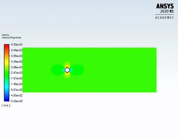
Fig. 40: Vortex shedding behind the cylinder using velocity contour animation plot for Reynolds number 100000

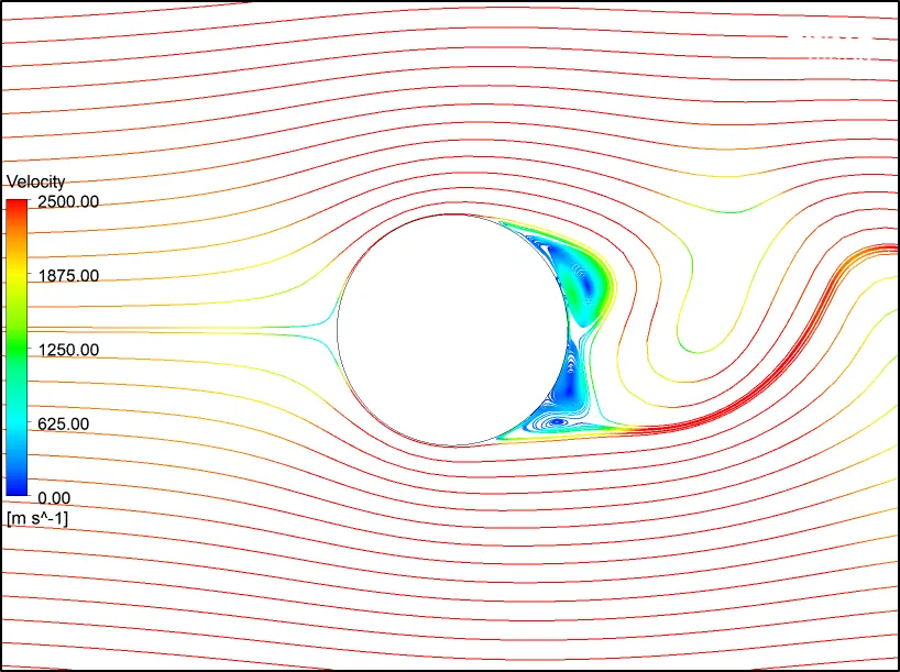
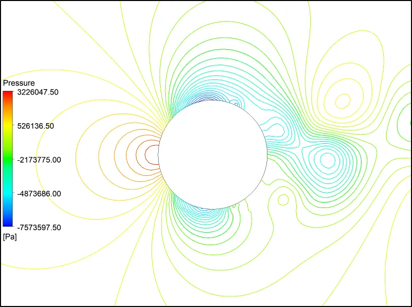Fig. 41: Streamline and static pressure contour (showing contour lines only) plots for Reynolds number 100000

Transient state:

For Reynolds number 100:

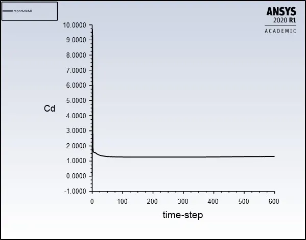
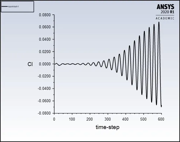Fig. 42: Coefficient of drag and lift on the cylinder wall for Reynolds number 100

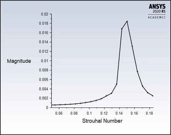
Fig. 43: Plot of Magnitude vs Strouhal Number for Reynolds number 100 with peak Strouhal number at 0.150

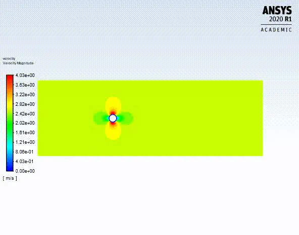
Fig. 44: Vortex shedding behind the cylinder using velocity contour animation plot for Reynolds number 100

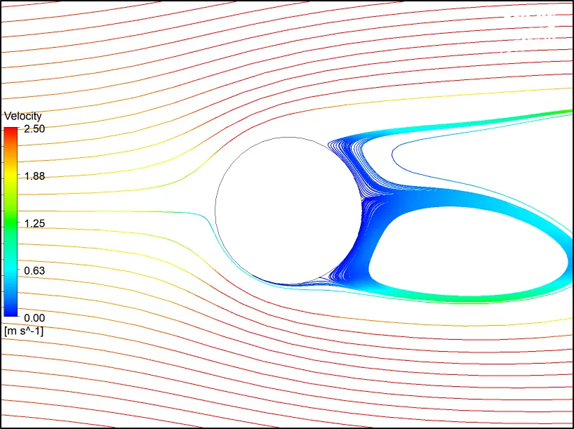
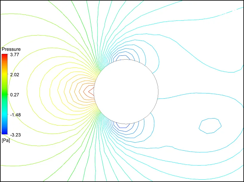Fig. 45: Streamline and static pressure contour (showing contour lines only) plots for Reynolds number 100

4. Discussion

The meshing approach chosen for this simulation was a quad-dominant mesh with near wall refinement in accordance to the boundary layer development. The results, especially for Reynolds number 10 and 100, have yielded an overall good agreement when compared against the experimental values reported by Wieselsberger (1922) [7], as can be seen in Table 19. The mesh quality attributes were in the range of "Good" and "Excellent" quality scales with regards to the values defined in Table 1. For Reynolds number 1000, 10000, and 100000, the Coefficient of Drag values show large variations between the current numerical analysis and the experimental values and this behaviour can be attributed to the fact that the boundary layer was transitioning from laminar to turbulent regime which is causing the separation point to move further along the surface of the cylinder in the downstream flow direction. This is contributed by the large variations in local pressure gradient, as can be seen in Fig. 35, Fig. 38 and Fig. 41, that leads to drastic changes in fluid flow forces from acceleration to deceleration and in turn slows down the flow of the fluid to respond accordingly. Since, there is interaction between the local pressure gradient with the boundary layer, the fluid flow loses momentum as a result of viscous friction and viscous losses thereby preventing build-up of sufficient momentum to overcome the resulting retarding force. Hence, the layers of fluid flow close to the wall experience a reversing change in the flow direction leading to separation. It must be noted that Reynolds number 10000 does experience a slightly higher drag coefficient value than Reynolds number 1000 despite no changes in the overall setup other than changing the velocity value corresponding to the same mentioned in Table 2.

Coefficient of Drag vs Reynolds number:

Reynolds Number	Coefficient of Drag(Cd) - Numerical Analysis	Coefficient of Drag(Cd) - Experimental Results	Absolute Difference (%)
10	3.3332	3.3553	0.6590
100 (steady state)	1.3721	1.3475	1.8255
100 (transient state)	1.3072	1.3475	2.9982
1000	1.4018	1.1939	17.4133
10000	1.4047	1.0286	36.5628
100000	0.8354	0.9537	12.4017

Table 19: Comparison of Coefficient of Drag values between Numerical Analysis and Experimental Results (reported by Wieselsberger (1922) [7]) for Reynolds number 10, 100, 1000, 10000 and 100000)

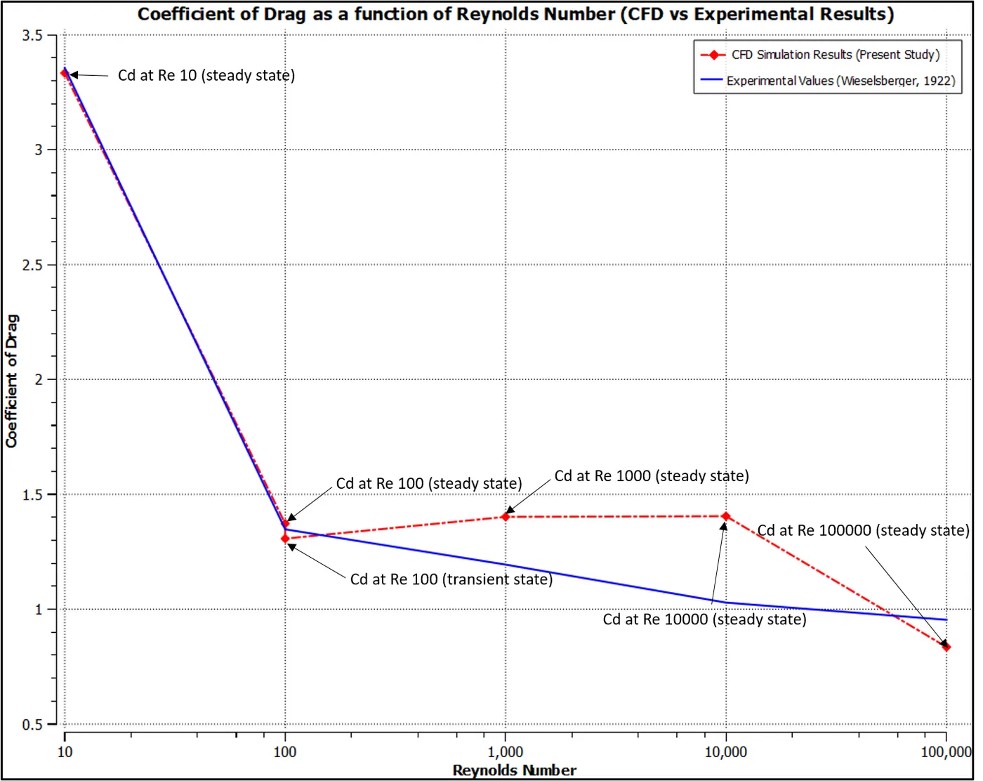
Fig. 46: Plot of Coefficient of Drag as a function of Reynolds number (CFD vs Experimental Results) for Re 10, 100 (steady and transient states), 1000, 10000, 100000

5.Conclusion

The numerical analysis for flow over a cylinder under both steady and unsteady conditions using laminar and k-`omega` SST turbulence model in ANSYS Fluent 2020 R1 was well understood. It was realised that based on the boundary layer development over the cylinder and use of an appropriate viscous model, a CFD model was able to replicate the expected physical phenomena of vortex shedding. Additionally, the Karman vortex street (laminar) observed at Reynolds number 100 in both steady and unsteady state gave a deeper understanding of the flow regime and demonstrated the capabilities of this mathematical model when validated against experimental results. This also implies that the selected material properties for the fluid viz., Density of 1 `(kg)/m^3`and Viscosity (or dynamic viscosity) of 0.05 `(kg)/(ms)`, have performed reasonably well in the preparation of the computational model. The k-`omega` SST turbulence model used for this simulation did show large variations in the prediction of coefficient of drag values, however, better correlation could be possible to achieve with an improved mesh refinement near the wall.

References

[1] Roshko, A. & Fiszdon, W. 1969 On the persistence of transition in the near-wake. SIAM J., pp. 607–616.

[2] A. Roshko, Perspectives on bluff body aerodynamics, Journal of Wind Engineering and Industrial Aerodynamics, Volume 49, Issues 1–3, December 1993, Pages 79-100, ISSN 0167-6105

[3] D.J. Tritton, Experiments on the flow past a circular cylinder at low Reynolds number, Journal of Fluid Mechanics, 6 (1959), pp. 547-567

[4] ZDRAVKOVICH, M. M., & BEARMAN, P. W. (1997). Flow around circular cylinders. vol 1, vol 1. Oxford, Oxford University Press.

[5] Roshko, A. (1954) On the Development of Turbulent Wakes from Vortex Streets. NACA Report 1191, National Advisory Committee for Aeronautics, Washington DC.

[6] Sumer, B. & Fredsoe, J. 1997, ‘Hydrodynamics around cylindrical structures’, Advanced Series on Ocean Engineering Volume 12, Department of Hydrodynamics and Water Resources, Technical University of Denmark.

[7] Wieselsberger, on the drag of circular cylinders, Physikalische Zeitschrift, vol. 22, 1992, pp. 219-224.