Week 9 - FVM Literature Review

1. Finite Volume Method

Finite Volume Method (FVM) can be defined as a discretization method that makes use of the integral formulation for the governing equations in accordance with the conservation laws. The manner in which FVM is implemented is explained as points of difference against Finite Difference Method (FDM), another discretization method, also highlighting the scope, advantages and drawbacks of these techniques in different scenarios in Section 2. Differences between Finite Volume Method and Finite Difference Method.

2. Differences between Finite Volume Method and Finite Difference Method

		Finite Volume Method (FVM)	Finite Difference Method (FDM)
1.	Grid Generation	Domain is divided into control volumes or cells with variable of interest located at the centroid of each control volume.	Domain is divided into points with each point representing variable of interest.
2.	Discretization	Differential form of governing equations are integrated over each control volume i.e., discretization is based on fluxes.	Differential form of governing equations are replaced by system of algebraic equations at each grid point, or in other words, discretization is based on derivatives.
3.	Laws of conservation	Conservation principles including mass, momentum and energy are maintained by definition.	Conservation laws are not preserved in all cases.
4.	Applicability	Structured and unstructured grids as shape of control volume does not impact conservation principles.	Structured grids in most cases.
5.	Examples of Numerical Schemes	Upwind Differencing, Hybrid Differencing, Power Law : Convection-Diffusion problems	Forward difference, backward difference, central difference
6.	Advantages	Robust in terms of performance with respect to challenging problems that cover both academia and industrial physical processes, cheap in regards to quick and reliable coding.	Easier implementation, availability of higher order schemes, and generally lower computational cost and improved efficiency over FVM for problems of similar nature with simpler grid structures.
7.	Disadvantages	Presence of false diffusion when lower order accuracy upwind schemes are preferred due to stability issues in higher order accurate schemes like central differencing, and difficulty to accomplish higher order schemes in comparison to FDM.	Use of mapping functions in methods like variable transformation technique is required when point(s) are not aligned along cartesian coordinates which becomes increasingly challenging with more complex geometrical features.
8.	Applications	Physical Problems: Evaluation of external aerodynamics features of aircraft bodies, analysis of different heat transfer modes and mechanisms when graphics processing unit (GPU) on a graphics card dissipates power within an enclosed domain, assessment of wells in petroleum engineering. Commercial Software(s): ANSYS CFX, ANSYS FLUENT, PHOENICS, STAR-CD, OpenFOAM	Physical Problems: Prediction of quantities based on models developed to study weather and its attributes, astrophysics applications, seismology. Commercial Software(s): No known commercially available software, although research codes have been developed for select physical problems.

Table 1: Differences between FVM and FDM

3. Interpolation schemes and flux limiters in Finite Volume Method

Interpolation schemes, with regards to FVM, can be outlined as methods of estimating values of variables at locations other than at nodal points, such as cell faces, for approximation of surface and volume integrals. Different types of interpolation schemes exist and can be used to fit different grid structures.

Flux limiters in FVM can be described as partial differential equations, typically employed and/or enabled in high resolution schemes for spatial derivatives, to reduce the occurrence of spurious oscillations or wiggles that tend to arise due to instabilities especially when shocks or discontinuities are also modelled in a given domain. In essence, the flux limiter, when defined correctly, aids high and low order schemes by resolving regions of smooth flow with high order accuracy while zones of shocks or discontinuities are reduced usually to first order accurate solutions.

In the following sub-section 3.1. 1D linear steady state heat conduction equation, the importance of linear interpolation scheme to calculate temperature flux at cell faces is justified, however flux limiter for the given problem would assume significance in a different application where high resolution schemes such as total variation diminishing (TVD) are used or can be defined when gradients approach 0 or 1 values representing sharp or smooth solutions respectively, requiring appropriate change in the resolution scheme for the fluxes.

3.1. 1D linear steady state heat conduction equation

Let us consider a 1D linear steady state heat conduction across a plate of thickness 'T'm, uniform cross-sectional area of 'A'`m^2` and heat generation of constant value 'S'`(kW)/m^3` such that temperature gradients in the x-direction are significant over the large dimensional values in y and z directions. The corresponding governing equation describing steady state heat conduction phenomena is mathematically expressed below as:

`(del)/(del x)(k*(del T)/(del x)) + S`; where (Eq. 1)

`k` represents thermal conductivity value

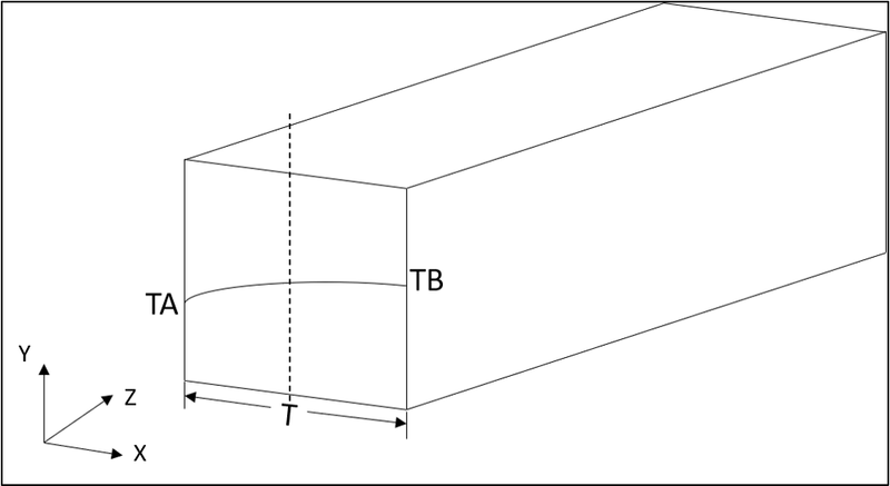
Fig. 1: 1D steady state heat conduction problem description

Step 1: Grid Generation

The given domain length is divided into 'n' equally sized control volumes resulting into the spacing between the centroids of each control volume as `delta x` and the distance between the centroid and the face of each control volume as half of `delta x` i.e., `(delta x)/2`, also illustrated in the figure below.

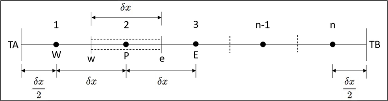
Fig. 2: Grid generation for 1D steady state heat conduction problem

Step 2: Discretization

Integration of differential form of governing equation over each control volume to yield a discretized equation at the centroid of the cell.

`int_(Delta V)((del)/(del x)(k*(del T)/(del x)))*dV + int_(Delta V)(S)*dV = 0`; where (Eq. 2)

The control volume, `dV`, can be expressed as the product of the surface area perpendicular to the direction of heat flow and the spacing between corresponding control volumes which can be mathematically formulated in the following equation:

`dV = A*dx`

It should be noted that the cross-sectional area and spacing between centroids of each control volumes are assumed as constants for simplicity i.e., (`A_e = A_w = A`) and (`delta x_e = delta x_w = delta x`) respectively wherein 'e' and 'w' represent east and west orientations of a control volume.

Simplifying (Eq. 2) and using the expression representing the control volume mathematical product; we get

`[k*A(del T)/(del x)]_w^e + overline S*Delta V = 0`, or

`(k*A(del T)/(del x))_e - (k*A(del T)/(del x))_w + overline S*Delta V = 0`; where (Eq. 3)

`overline S` represents average value of source term, S, over each control volume

Eq. 3 represents that the temperature flux leaving the east face subtracted by the temperature flux entering the west face is equal to the generation of temperature i.e., a balance equation for temperature is constituted over each control volume.

In order to calculate gradients and therefore fluxes at control volume faces, approximate distribution of temperature between nodal points needs to be used, in this case being linear approximation or interpolation using central differencing for demonstration purposes although other forms of approximation can also be used. Linearly interpolated values for thermal conductivity at east and west faces can be expressed mathematically as:

`k_w = (k_W+k_P)/2`, and (Eq. 4.a)

`k_e = (k_P+k_E)/2` (Eq. 4.b)

Temperature fluxes are then mathematically evaluated as:

`(k*A(del T)/(del x))_e = k_e*A*((T_E-T_P)/(delta x_(PE)))`, and (Eq. 5)

`(k*A(del T)/(del x))_w = k_w*A*((T_P-T_W)/(delta x_(WP)))` (Eq. 6)

The source term is often expressed as a function of the dependent variable, in this case temperature, owing to its definition with respect to practical situations and the same can be expressed in a linearised form as shown below:

`overline S*Delta V = S_u + S_p*T_p` (Eq. 7)

Substitution of Eq. 4.a and Eq. 4.b into Eq. 6 and Eq. 5 respectively, and then Eq. 5 and Eq. 6 into Eq. 3; we get

`(((k_e)/(delta x_(PE))+(k_w)/(delta x_(WP)))*A - S_p)*T_P = ((k_w)/(delta x_(WP))*A)*T_W + ((k_e)/(delta x_(PE))*A)*T_E + S_u` (Eq. 8)

Eq. 8 can be rewritten using coefficients of `T_P`,`T_W` and `T_E` as `a_P`,`a_W` and `a_E` respectively using the following expression:

`a_P*T_P = a_W*T_W + a_E*T_E + S_u`; where (Eq. 9)

`a_W`	`a_E`	`a_P`
`(k_w)/(delta x_(WP))*A`	`(k_e)/(delta x_(PE))*A`	`a_W + a_E - S_p`

Eq. 9 and Eq. 7 represent the discretised form of a general steady state transport equation, in this case, 1D linear heat conduction equation.

Eq. 8 above is valid for all discretized nodal points except at the boundaries which either represents known or unknown values depending on the direction of flow, in this case transfer of heat. Assuming the direction of heat flow from left to right in Fig. 1 along x-direction such that temperature and thermal conductivity on the boundary at the west of first node, point A, is known, then temperature at nodal point 1 can be estimated by linear approximation in the following manner:

Integrating the differential form of governing equation over the control volume representing nodal point 1 and the boundary at its west yields the same form as Eq. 3 except now the spacing between the centroid of the cell and the boundary is halved i.e., `(delta x)/2` as shown below:

`(k_e*A*((T_E-T_P)/(delta x))) - (k_A*A*((T_P-T_A)/((delta x)/2))) + overline S*Delta V = 0`, which in discretized form can be rewritten as Eq. 9, where (Eq. 10)

`a_W`	`a_E`	`a_P`	`S_p`	`S_u`
0	`(k_e)/(delta x)*A`	`a_W + a_E - S_p`	`-(2*k_A)/(delta x)*A`	`overline S*Delta V + (2*k_A)/(delta x)*T_A`

Similarly, at nodal point n, the differential form of governing equation over the control volume representing the last nodal point and the boundary at its east, point B, also yields the same form as Eq. 3 with similar spacing value between the centroid of the cell and the boundary as `(delta x)/2`, only this time the temperature on the east face of the control volume is known and can be mathematically expressed below:

`(k_B*A*((T_B-T_P)/((delta x)/2))) - (k_w*A*((T_P-T_W)/(delta x))) + overline S*Delta V = 0`, which in discretized form can be rewritten as Eq. 9, where (Eq. 11)

`a_W`	`a_E`	`a_P`	`S_p`	`S_u`
`(k_w)/(delta x)*A`	0	`a_W + a_E - S_p`	`-(2*k_B)/(delta x)*A`	`overline S*Delta V + (2*k_B)/(delta x)*T_B`

Step 3: Solution of Equations

Discretized form of equations for control volumes at the boundaries in Eq. 10 and Eq. 11 and for control volumes in the rest of the domain in Eq. 9 represent a system of linear algebraic equations which can then be solved using appropriate matrix solution techniques to obtain distribution of temperature along subsequent nodal points.