Week 5: Prandtl Meyer Shock problem
1. Introduction
Supersonic fluid flow of typically air, characterised by a value of Mach number greater than 1, generally tends to produce oblique supersonic wave(s) around the object it flows over and forms an important and unique set of behavioural aspects in practical scenarios dealing with compressible flow. A historical detour to the days of the first Concorde flight in 1976, would be an apt reminder into the much talked about "sonic boom" reported as an explosive sound which principally speaking was an outburst of immensely huge amounts of sound energy (pressure waves) created as a result of disturbances (waves) to fluid flow generated by the flight travelling faster than the speed of sound in the same medium in such a way that the wave motions were restricted from propagating upstream whereby they merge over a short distance immediately upfront of the aircraft leading to formation of a thin wave front, also called as a shock wave or quite simply shock. These shock waves can be well-identified as "wedge and cone flows" which is a classification of "oblique shock waves" under the previously mentioned oblique supersonic wave(s). The main reason behind specifying supersonic wave(s) as oblique is because most of their formation(s) on the surface of a particular object travelling at supersonic speeds are generally inclined at an oblique angle with respect to the incoming flow barring the exception of a normal shock wave which is perpendicularly aligned. Oblique shock waves are known to occur when the incoming supersonic flow gets deflected by a concave surface in its direction such that it gets "turned into itself" while oblique expansion waves take place when the same incoming supersonic flow encounters a convex surface such that beyond it an expansion region gets created or it gets "turned away from itself". The oblique supersonic wave(s) also have a significant effect on the flow properties wherein for oblique shock waves, an increase in static properties viz., pressure, temperature and density, increase in entropy and decrease in Mach number and total pressure is observed and also to be discontinuous or marked by abrupt changes while conversely for oblique expansion wave(s), a decrease in static properties, decrease in entropy and increase in Mach number and total pressure is noticed but the variations take place more gradually or smoothly over the concerned region.
The aim of this challenge was to perform two-dimensional, steady-state simulations, using the default physical model without turbulence modelling to solve the compressible form of Navier-Stokes equations for an inviscid, supersonic flow moving over a surface consisting of a convex corner to visualise the oblique expansion waves, also commonly known as the Prandtl-Meyer expansion wave, and compute flow properties over the entire region. The analysis involved verification and validation of the computational model against the exact, analytical solutions for mach number, pressure, density, temperature and velocity at the outlet, as reported by John D. Anderson, Jr. in [1], using both the default base grid size settings, mentioned in [1], as well as computing results for the same flow properties using the sub-grid scale (SGS)-based adaptive mesh refinement (AMR) for three different temperature dependent sub-grid criterion values and two different maximum embedding level along with stating the total cell count and mesh quality attributes like skewness, non-orthogonality, and aspect ratio, and evaluating the profiles for the x-component of velocity in all cases.
2. Method
The typical approach adopted to performing numerical simulations in CONVERGE CFD involves the following steps:
- Creating a new folder dedicated to running the concerned project inside a user-preferred directory.
- Setting up the relevant case file(s) in Converge Studio v3.0 that involves creation of the fluid volume domain, setting up the required application type, choosing material and its state (gas, liquid, parcel or solid) for which simulation is to be performed along with the requisite properties, defining simulation parameters such as solver types, monitor variables, run time variables, and convergence tolerances, defining region(s), boundary conditions and initial conditions, specifying the physical models whose equations are intended to be solved, determining and allocating the base grid size values as well as any other refinements, and lastly selecting the variables for post-processing at the required time intervals (in terms of cycles for steady-state) along with any hidden parameters or UDF selection as part of advanced parameters.
- Saving the case file(s) and exporting the input files into the folder created for running the concerned project which typically includes 'boundary.in' for the various boundary conditions, 'material_state.dat' where material_state points to either 'gas', 'liquid', 'parcel' or 'solid', 'initialize.in' specifying initial conditions, 'inputs.in' defining the various input conditions and file writing intervals, 'monitor_steady_state.in' to assign monitor variables for the steady state simulation, 'post.in' for the different post-processing variables, 'solver.in' describing the solver chosen and its equations, and 'surface.dat' containing datasets about the surface while other input files with respect to the state of the material, thermal properties and species may also be part of the exporting process and should be ensured that they are selected for the simulation to run.
- Running the simulation in a Cygwin64 terminal window.
- Post-converting 3D output data by navigating to the output folder created within the same project folder during the simulation run or from the 'Post-Processing 3D' button in Converge Studio v3.0.
The simulation run and post-converting processes were executed using Linux-type commands in a Cygwin64 terminal window as shown below:
i) Change directory to the project containing the relevant case file(s):
cd "PATH_TO_CONCERNED_PROJECT_FOLDER"
ii) Confirm the contents of the project for the exported input files:
ls
iii) Performing simulation run with the converge executable application on multiple processors (in this case, 4) using mpiexec executable file in the background (by adding ampersand operator) along with posting output into a logfile:
mpiexec.exe -n 4 converge.exe restricted </dev/null> logfile &
iv) Checking for simulation status with regards to completion or errors:
tail logfile
v) Post-converting the 3D output data files using the 'post_convert_30_msmpi_64' utility on multiple processors (in this case, 4) using mpiexec executable file from within the output folder of the project containing the exported input files:
cd output
mpiexec.exe -n 4 post_convert_30_msmpi_64
2.1 Modelling
The computational domain for performing steady state simulation of supersonic air flow through a centered expansion wave was modelled in Converge Studio v3.0. The length of the domain was provided as 65m in the direction of flow, from the inlet to the outlet, with the convex corner located at a position of 10m, again from the inlet, and the height thereafter varying as a function of spatial x-coordinate i.e., `h = 40m` for `0<=x<=10m` while `h = 40 + (x-10)*tan(theta)` for `10<=x<=65m`. The basic element entity in CONVERGE is denoted by a triangle which would be visible by clicking on any of the surfaces of the recently drawn model and in order to demarcate boundaries, the corresponding triangles needed to be grouped together. The process of grouping and creating new boundaries began with clicking on the 'Boundary' button under the 'Geometry' dock which was followed by clicking on the '+' symbol from which the pop-out message would read as 'Create a new boundary.' leading to the 'Boundary definition' window to open in which the option 'Create multiple boundaries' was checked with the number of boundaries set to 4, in this case, followed by lastly grouping the triangles that constitute a given surface and naming them accordingly, such as 'Inlet', 'Outlet', 'TopBottomSlipWalls', 'Front2D' and 'Back2D' as illustrated in Fig. 1. Moreover, the normal from each of the triangular surface is required to point towards the fluid domain which was ensured by first visualising the same using the 'Normal toggle' button accessible in the 'View Toolbar' and depending on the direction along which the normal is pointing, a decision was taken by clicking on the 'Normal' tab within the 'Transform' button under the 'Geometry' dock and selecting the suitable option from one of the three 'Transform Normal Options' followed by clicking on the 'Apply' button. At this stage and for the given numerical analysis, the modelling requirements were achieved, however, to validate if the model was clean i.e., it contains no intersecting edges, overlapping triangles or any other form of geometrical constraints, a check was performed by clicking on the 'Find' button in the 'Diagnosis' dock to observe for any anomalous 'Problem Triangles' and rectify the same.
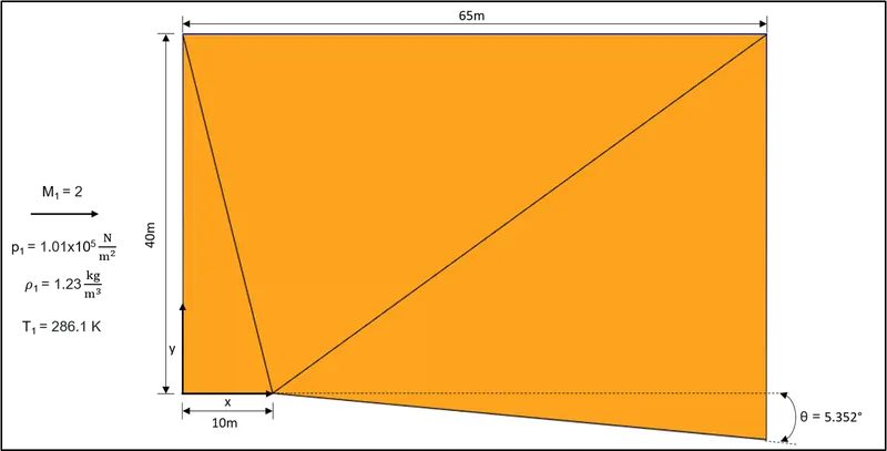
Fig. 1: Fluid Volume Model and Boundary Conditions regions in two-dimensional space (Image recreated for this study as illustrated by John D. Anderson, Jr., in [1] with no intention to infringe on the copyrights of the original author and/or his publication)
2.2 Meshing
The meshing approach adopted for the given computational domain was developed to maintain the meshing quality attributes viz., aspect ratio, skewness, and non-orthogonality as outlined in the CONVERGE 3.0 Manual [2] provided in the following table:
|
Aspect Ratio |
1 (Ideal Value) |
||
|
Skewness |
0° (Ideal Value) |
< 70° (Acceptable) |
`>=` 90° (Likely to cause simulation failure) |
|
Non-Orthogonality |
0° (Ideal Value) |
< 70° (Acceptable) |
`>=` 90° (Likely to cause simulation failure) |
Table 1: Mesh Quality Attributes as defined in the CONVERGE 3.0 Manual [2]
The reason for pursuing the above mentioned mesh quality attributes, as specified in Table 1, can be ascertained on the fact that whether the discretized domain was likely to create convergence issues during the solution process and also to identify areas in the mesh where the statistics can be improved based on the underlying physics. In Section 2.5.2 Sub-grid scale (SGS)-based adaptive mesh refinement (AMR) using temperature dependent sub-grid criterion, detailed discussion about the different meshes that were prepared and their mesh qualities has been highlighted.
2.3 CFD Simulation Setup, Boundary Conditions and Monitoring Variables
The simulations on all meshes was performed using the default physical model consisting of no turbulence equations. A brief description into the working of the default physical model is provided below:
2.3.1 Default physical model
The default physical model can be described as the solution of the governing fluid equation viz., Navier-Stokes equations for a domain, in this case, discretized using the finite volume approach, without the presence of turbulence terms. The Navier-Stokes equations define the fluid flow properties such as velocity, pressure, density, temperature, viscosity, energy, etc., within a given physical domain. Additionally, the Navier-Stokes equations are developed with regards to the laws of conservation that states the net mass flow across a system is zero (Conservation of mass) and that the momentum within the same system (or control volume) is constant (Conservation of momentum). Since, energy is also a variable of assessment for the given numerical analysis, then according to the first law of thermodynamics, total heat gain of a system is equal to the sum of heat added to the system and work done on the same system.
2.3.1.1 Setup of the default physical model:
To use the default physical model in Converge Studio v3.0, we navigate to Physical Models option in the Case Setup tree and uncheck 'Turbulence modeling' to prevent inclusion of turbulence terms in the solution of governing flow equations.
2.3.2 Boundary Conditions and Monitoring Variables
The different boundary conditions for simulation of supersonic air flow through a centered expansion wave is described in Table 2. Since, the given numerical problem involves modelling of two-dimensional supersonic inviscid flow, it was important to ensure that the surface boundary conditions are coupled into the flow-field calculation such that the same supersonic inviscid flow can adapt to the surface over which it would be flowing. The setup in the given numerical simulation mimics the configuration adopted by John D. Anderson, Jr. in [1] wherein the 'Inlet' boundary surface is defined using Dirichlet boundary conditions, which is also recommended in the CONVERGE 3.0 Manual [2] for supersonic INFLOW boundaries, to allow for fixed condition based values to be stated i.e., static pressure value of `1.01*10^5 N/m^2`, velocity magnitude of 678m/s along the x-component, and temperature value of 286.1K while the 'Outlet' boundary surface is described using Neumann boundary conditions that evaluates the derivatives for the previously mentioned flow properties, more specifically zero-gradient along the normal orientation, as their values were required to be obtained from the numerical simulation barring the 'Temperature Backflow' parameter which was required to be specified, also suggested in the CONVERGE 3.0 Manual [2] as flow reaches the OUTFLOW boundary, in this case using Dirichlet boundary condition of 300K, deemed to be a reasonably realistic value while also ensuring convergence. The top and bottom walls of the given domain were modelled as slip walls, also a special case of the Neumann boundary conditions as specified in the CONVERGE 3.0 Manual [2], which for the velocity boundary condition sets the components of the stress tensor, tangential to the wall, to 0 or to put it simply, the velocity component parallel to the wall has a finite value but its normal component and the normal derivative of the velocity component parallel to the wall are set to 0 thereby further implying that the viscous effects is almost negligible or that the flow across the top and bottom wall surfaces is inviscid.
|
Names |
Inlet |
Front2D |
Back2D |
TopBottomSlipWalls |
Outlet |
|
Type |
INFLOW |
TWO_D |
TWO_D |
WALL |
OUTFLOW |
|
Pressure Boundary Condition |
Specified Value (DI) |
-- |
-- |
-- |
Zero normal gradient (NE) |
|
Pressure Magnitude (Pa) |
101001.0 |
-- |
-- |
-- |
-- |
|
Velocity Boundary Condition |
Specified Value (DI) |
-- |
-- |
-- |
Zero normal gradient (NE) |
|
Velocity Magnitude (m/s) |
(u v w) `-=` (678 0 0) |
-- |
-- |
-- |
-- |
|
Temperature Boundary Condition |
Specified Value (DI) |
-- | -- |
Zero normal gradient (NE) |
-- |
|
Temperature Backflow |
-- |
-- | -- |
-- |
Specified Value (DI) |
|
Temperature Magnitude (K) |
286.1 |
-- |
-- |
-- |
300 |
|
Species Boundary Condition |
Specified Value (DI) |
-- |
-- |
-- |
Specified Value (DI) |
|
Species Name: `O_2` |
0.23 |
-- |
-- |
-- |
0.23 |
|
Species Name: `N_2` |
0.77 |
-- |
-- |
-- |
0.77 |
|
Wall motion type |
-- |
-- |
-- |
Stationary |
-- |
|
Surface Movement |
-- |
-- |
-- |
Fixed, Slip |
-- |
Table 2: Boundary Conditions for simulation of supersonic air flow through a centered expansion wave defined using the 'Boundary' sub-option of the 'Boundary Conditions' under the 'Case Setup' tree
For the given problem, the simulation was chosen as 'Gas simulation' enabled in the 'Materials' option in the 'Case Setup' tree with 'Predefined mixtures' set to 'Air' and 'Species (not in mech.dat)' option enabled to utilise the mass fraction values of `O_2` and `N_2` as they represent the major constituting species in air by mass fraction. Since, 'Gas simulation' option was checked in the 'Materials' option, an equation of state was required to be defined that formulates a coupling relationship between the different state variables such as density and physical conditions such as pressure and temperature to depict the state of matter. In the given numerical analysis, the Redlich-Kwong (RK) cubic equation of state was set to in the 'Equation of state' drop-down menu with its default values of critical temperature (`T_c`) and critical pressure (`p_c`) retained at '133.0 K' and '3770000.0 Pa' respectively as it is a simpler form of representation in comparison to the Redlich-Kwong-Soave and Peng-Robinson set of equations but more accurate than the ideal gas law which works best for gases at low pressures, however, at higher pressures tends to report huge deviations in its predictions as it assumes that the molecular volume is very small and that neither attraction or repulsion exists between the molecules which is not true in the case of real gases. Additionally, the real gas properties would behave as a function of temperature which was again set to as the default option in the 'Gas simulation' window. The values of 'Turbulent Prandtl number' and 'Turbulent Schmidt number' were left unchanged at their default values of 0.9 and 0.78 respectively.
During the solution process, a monitor variable was created to observe the behaviour of flow-field variables viz., mach number, density, static pressure and temperature by selecting 'AVG_VELOCITY' from the list of 'Monitor Variables' available by default with 'Target Type' and 'Target' set to 'Boundary' and 'Outlet' respectively and file name as 'mass_avg_flow.out' from the 'File Name' drop-down menu. The settings of the remaining parameters for the reporting of the monitor plots included entering values of 'Minimum number of cycles to be executed for the steady-state solver' and 'Sample size, cyc' such that the given solution would run for at least 15000 cycles regardless of whether a state of convergence would have been achieved prior to it and 1000 number of samples to decide if the concerned variable has reached steady-state condition with 'Monitor start delay, cyc' having a value of 0 before clicking on the 'Validate' and 'OK' buttons.
2.4 Post-Processing
The extended part of the solution process using Converge Studio v3.0 included selecting the variables of interest whose quantitative and qualitative aspects would highlight the behaviour of the flow, in this case within the given fluid domain, under different circumstances and they were chosen by clicking on the 'Post variable selection' sub-option of the 'Output/Post-Processing' setting under the 'Case Setup' tree and checking the boxes 'Density', 'Mesh Quality', 'Pressure', 'Temperature', 'Velocity' and 'Cell Mach number' in the 'Typical Variables' section and 'Region ID' (normally enabled by default) in the 'Geometry/Location' section of the 'Typical Variables/Geometry' tab and adding 'Mass Fraction' under 'Species' section of the 'Species/Passive' tab for `O_2` and `N_2` species with respect to the concerned numerical analysis. Visualising the different flow variable quantities in two-dimensional space in ParaView required the creation of a slice of the given fluid domain by using the "Slice" tool in the 'Commons' toolbar typically located above the 'Pipeline Browser' window based on default layout settings and choosing 'Z Normal' under 'Plane Parameters' section to align the plane normal to the z-axis direction such that the entire domain was viewed in the direction of flow followed by unchecking the 'Show Plane' and 'Triangulate the slice' boxes for disabling the viewing of the plane borders and production of triangles in the output respectively. Plotting the velocity (x and y components), temperature, pressure, density, and mach number profiles at x=12.928m and velocity (x-component) profiles at different space intervals from the inlet of the given domain for both the verification and validation cases were performed by using ParaView's in-built "plot over line" tool. The "plot over line" tool was accessed by clicking on 'Filters' present in the data analysis group, followed by entering the coordinates as seen in Table 3, Table 4, Table 5, Table 6 and Table 7 before clicking on the "Apply" button to view the said profiles.
It was ensured that the last time-step size of the simulation run was selected to view the velocity (x and y components), velocity magnitude, temperature, pressure, density, and mach number profile results. Additionally, velocity, pressure , temperature, density and mach number field plots were created to view the development of the flow field characteristics across the fluid domain. Legends, titles, and x and y labels were added for better understanding of the graphical representations.
|
Line 1 |
x |
y |
z |
|
Point 1 |
12.928 |
4.878243163 |
0 |
|
Point 2 |
12.928 |
45.15254592895508 |
0 |
Table 3: Line Coordinates for viewing the velocity (x and y components), temperature, pressure, density, and mach number profiles at x = 12.928m
|
Line 2 |
x |
y |
z |
|
Point 1 |
16.17 |
4.574523998 |
0 |
|
Point 2 |
16.17 |
45.15254592895508 |
0 |
Table 4: Line Coordinates for viewing the velocity (x component) profiles at x = 16.17m
|
Line 3 |
x |
y |
z |
|
Point 1 |
32.21 |
3.071854227 |
0 |
|
Point 2 |
32.21 |
45.15254592895508 |
0 |
Table 5: Line Coordinates for viewing the velocity (x component) profiles at x = 32.21m
|
Line 4 |
x |
y |
z |
|
Point 1 |
48.99 |
1.499859292 |
0 |
|
Point 2 |
48.99 |
45.15254592895508 |
0 |
Table 6: Line Coordinates for viewing the velocity (x component) profiles at x = 48.99m
|
Line 1 |
x |
y |
z |
|
Point 1 |
65 |
0 |
0 |
|
Point 2 |
65 |
27.02157241 |
0 |
Table 7: Line Coordinates for viewing the velocity (x and y components), temperature, pressure, density, and mach number values at x = 65m
To save an animation file of the different field plots, the option 'Save Animation' was accessed under the 'File' menu and clicked on followed by choosing the appropriate settings under the different sections such as 'Size and Scaling', 'Coloring', 'Compression Options' and 'Animation Options' to name a few, assigning an appropriate name to the animation file, in this case by the variable whose field plot is being indicated before clicking on the 'OK' button.
2.5.1 Comparison of baseline numerical simulation results and exact, analytical solution
2.5.1.1 Exact, Analytical solution
Assuming a calorically perfect gas, an exact, analytical solution for the flow conditions behind the expansion wave can be determined starting with the following relation:
`f_2 = f_1 + theta`; where (Eq. 1)
`f` represents the Prandtl-Meyer function, and
`theta` as the flow deflection angle equating to a value of 5.352° (as seen in Fig. 1)
Also, the Prandtl-Meyer function, `f`, is dependent on mach number, `M` and ratio of specific heats, `gamma`, as expressed mathematically below:
`f = sqrt((gamma + 1)/(gamma - 1))tan^-1sqrt((gamma - 1)/(gamma + 1)*(M^2-1))-tan^-1sqrt(M^2-1)` (Eq. 2)
The procedure to evaluate the analytical solution can be described using the steps mentioned below:
- Calculate `f_1` from known `M_1` using (Eq. 2) for region 1.
- Calculate `f_2` using value of `f_1` from previous step and substituting the value of `theta` into (Eq. 1).
- Determine `M_2` from (Eq. 2) by substituting the value of `f_2` into (Eq. 2) for region 2.
- Evaluate pressure, temperature and density values from (Eq. 3), (Eq. 4) and (Eq. 5), shown below, which are formulated with respect to isentropic flow conditions.
`p_2 = p_1{(1+[(gamma-1)/2]*M_1^2)/(1+[(gamma-1)/2]*M_2^2)}^(gamma/(gamma - 1))` (Eq. 3)
`T_2 = T_1(1+[(gamma-1)/2]*M_1^2)/(1+[(gamma-1)/2]*M_2^2)` (Eq. 4)
`rho_2 = p_2/(R*T_2)` (Eq. 5)
2.5.1.2 Numerical Simulation
This particular sub-section deals with the setup of the numerical simulation with regards to the spatial grid generation and initial conditions followed by comparison of results obtained against the resulting quantitative values from the isentropic flow relations in Section 2.5.1.1 Exact, Analytical solution.
Spatial grid generation:
The grid setup by John D. Anderson, Jr. in [1] makes use of a boundary-fitted coordinate system so as to transform the bottom surface beyond the convex corner in the direction of flow into a rectangular grid with respect to a finite difference solution. This implied that the physical x-y plane transformed to a `xi-eta` computational plane with the coordinates varying from 0 to L along the `xi` direction, similar to the coordinates along the x direction in the cartesian coordinate system, however, for `eta`, the coordinates varied from 0 to 1 as opposed to 0 to H along the y direction in the cartesian coordinate system with the former dependent on the position of the vertical spacing, `h`, which essentially was a function of the horizontal spatial position i.e., `h(x)`. The meshing approach adopted by CONVERGE, a finite volume CFD software package, is a Cartesian cut-cell grid method, which is a body-fitted mesh generated at run-time that attempts to create a perfect mesh alignment with the concerned geometry such that easier formation and better accuracy is ensured by cutting volume cells at the wall instead of stretching and compressing them and therefore, a similar grid configuration as that performed by John D. Anderson, Jr. in [1] could not be reconstructed. Thus, the consequent grid generation had similar downstream marching step size i.e., `Delta xi = Delta x`, of 0.818m as that determined by John D. Anderson, Jr. in [1] for Courant number of 0.5, but the same value of 0.818m was also considered in the case of the vertical spatial settings i.e., `Delta y` for the setup in CONVERGE, which was different to that evaluated for the finite difference solution (`Delta eta`).
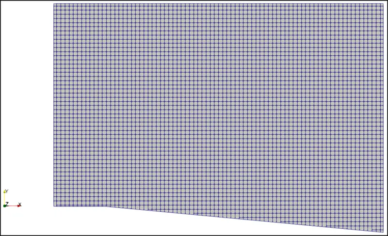
Fig. 2: Baseline Mesh (two-dimensional sliced view)
Initial conditions:
The initial conditions for the numerical simulation are the same as the velocity, temperature and pressure boundary conditions at the 'Inlet' boundary surface as tabulated in Table 2 which is also mentioned by John D. Anderson, Jr. in [1].
Comparison of numerical simulation results using baseline mesh against exact, analytical solution:
Fig. 3 provides a comparison between results obtained from numerical simulation using baseline mesh and exact, analytical solution for x-coordinate position at 12.928m with regards to the velocity (x and y components), temperature, pressure, density, and mach number profiles wherein it can be observed that a reasonable agreement was achieved in all of the flow-field parameters with very small differences in the direction of maximum gradient change i.e., y-axis orientation, except at the location close to the wall boundary surface along the expansion corner. Similarly, Fig. 4 represents the x-component of velocity profiles at x-coordinate positions of 0m, 16.17m, 32.21m and 48.99m as well as its comparison between the exact, analytical solution and numerical simulation using baseline mesh, however, certain key differences can be noted at the corresponding distance intervals after the expansion corner. The x-coordinate position of 16.17m reveals that the variations between the predicted x-component of velocity and exact, analytical solution are significant in the region occupied within the wave i.e., in between the leading and trailing edges of expansion wave, and beyond the wave and this maybe attributed to the consequence of fewer number of grid points which can deal with the expected and immediate changes experienced in and around the vicinity of the expansion corner, acting as a singular point, leading to less accurate modelling of the wave in this zone. This behaviour is noticeable for x-coordinate positions located close to the expansion corner and considerably reduces as the numerical solution moves further downstream whereby the expansion wave gets wider as well as the distance between the wall boundary surface along the expansion corner and the trailing edge of the expansion wave becomes larger indicating reasonably improved agreement between the said profiles. It should be noted that the exact, analytical solution in Fig. 4 was referenced from a similar image presented by John D. Anderson, Jr. in [1] for which the values were not found to be tabulated, unlike in Fig. 3 whose flow-field properties were captured in a tabular format at x-coordinate position of 12.928m, and therefore, a certain degree of error may exist as a result of the visually driven approximation process. Table 8 highlights a percentage-based comparison between the numerically simulated values of flow-field parameters at the outlet, averaged quantities in the region occupied by the trailing edge of the expansion wave and the wall boundary surface along the expansion corner, and their analytical counterparts as estimated from (Eq. 1) to (Eq. 5) signifying reasonably good agreement between them.
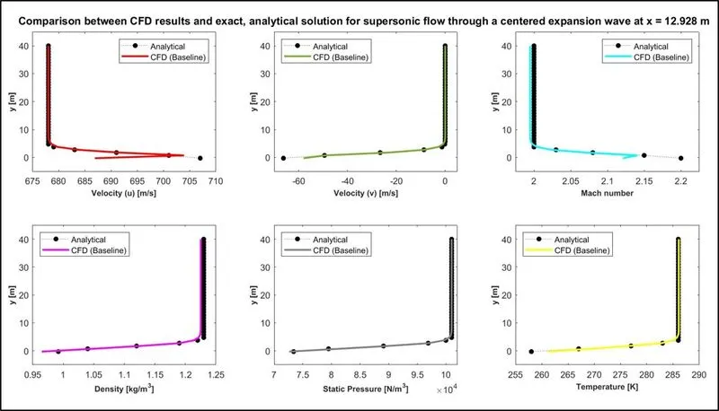
Fig. 3: Comparison between CFD results using baseline mesh and exact, analytical solution of different flow properties for supersonic flow through a centered expansion wave at x = 12.928m from inlet boundary surface
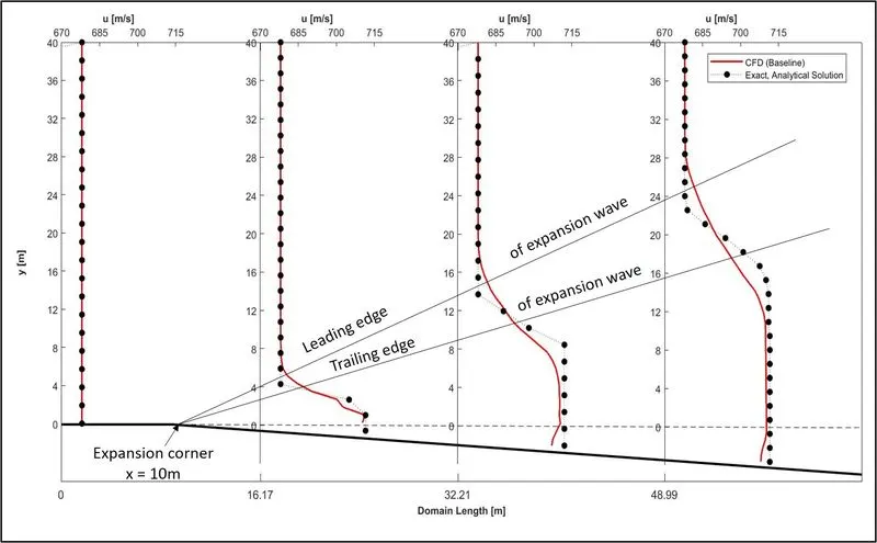
Fig. 4: Comparison between CFD results using baseline mesh and exact, analytical solution of x-component of velocity for supersonic flow through a centered expansion wave at x = 0m, 16.17m, 32.21m and 48.99m from inlet boundary surface (Adapted from [1] based on current numerical simulation]
| Flow-field parameters | Exact, Analytical Solution | Numerical Simulation (Baseline Mesh) | % error |
| Mach Number (`M_2`) | 2.2 | 2.189136 | -0.4938 |
| Static Pressure (`p_2`) (`N/m^2`) | 73900 | 74285.28 | 0.52135 |
| Density (`rho_2`) (`(kg)/m^3`) | 0.984 | 0.983785 | -0.02185 |
| Temperature (`T_2`) (`K`) | 262 | 262.0796 | 0.03038 |
| Velocity (u) (`m/s`) | 710 | 709.5199 | -0.06762 |
| Velocity (v) (`m/s`) | -66.5 | -65.6608 | -1.2619 |
Table 8: Percentage error comparison between predicted values of flow-field parameters using baseline mesh and exact, analytical solutions
2.5.2 Sub-grid scale (SGS)-based adaptive mesh refinement (AMR) using temperature dependent sub-grid criterion
From the CONVERGE 3.0 Manual [2], the mathematical formulation relating the embed size with the base grid size based on embed scale can be given by:
`embed = (base grid)/(2^(EMBED SCALE))`; where (Eq. 6)
`base grid` is the Base Grid Size defined for every element across the domain,
`EMBED SCALE` (or, in this case, maximum embedding level), is the scaling parameter by which the base grid size is to be refined either at the selected boundary, geometrical shape or region, and
`embed` is the scaled down or refined grid size
In the given numerical simulation, the approach adopted towards altering grid resolution is performed by using AMR and more specifically of the type SGS-based with the condition dependent on the temperature parameter. The principle involved with the SGS-based AMR is to refine a section of the `base grid` wherein maximum variations in the quantity of interest are known to occur, in this case temperature, dependent on the underlying physics such as the expansion fan region for the supersonic air flow through a centered expansion wave. This implies that a higher grid resolution is achievable wherein the flow field is under-resolved with the sub-grid field being the largest, in other words the curvature [gradient] of temperature, in this case, is the highest, or the quantity of interest suffices the embed criteria. Table 9 highlights the different mesh configurations employed in order to resolve the expansion fan region for supersonic air flow through a centered expansion wave based on altering the sub-grid criterion and maximum embedding level values.
|
Mesh |
dx (m) |
dy (m) |
dz (m) |
Sub-grid criterion (K) | Max Embedding Level |
|
1 |
0.818 |
0.818 |
1 |
0.25 | 2 |
|
2 |
0.818 |
0.818 |
1 |
0.025 | 2 |
|
3 |
0.818 |
0.818 |
1 |
0.0025 | 2 |
|
4 |
0.818 |
0.818 |
1 |
0.025 | 3 |
|
5 |
0.818 |
0.818 |
1 |
0.025 | 4 |
Table 9: Mesh sizes representing spatial grid settings across each of the three-directional axes, sub-grid criterion based on temperature (in K) and max embedding level values
Mesh 1:
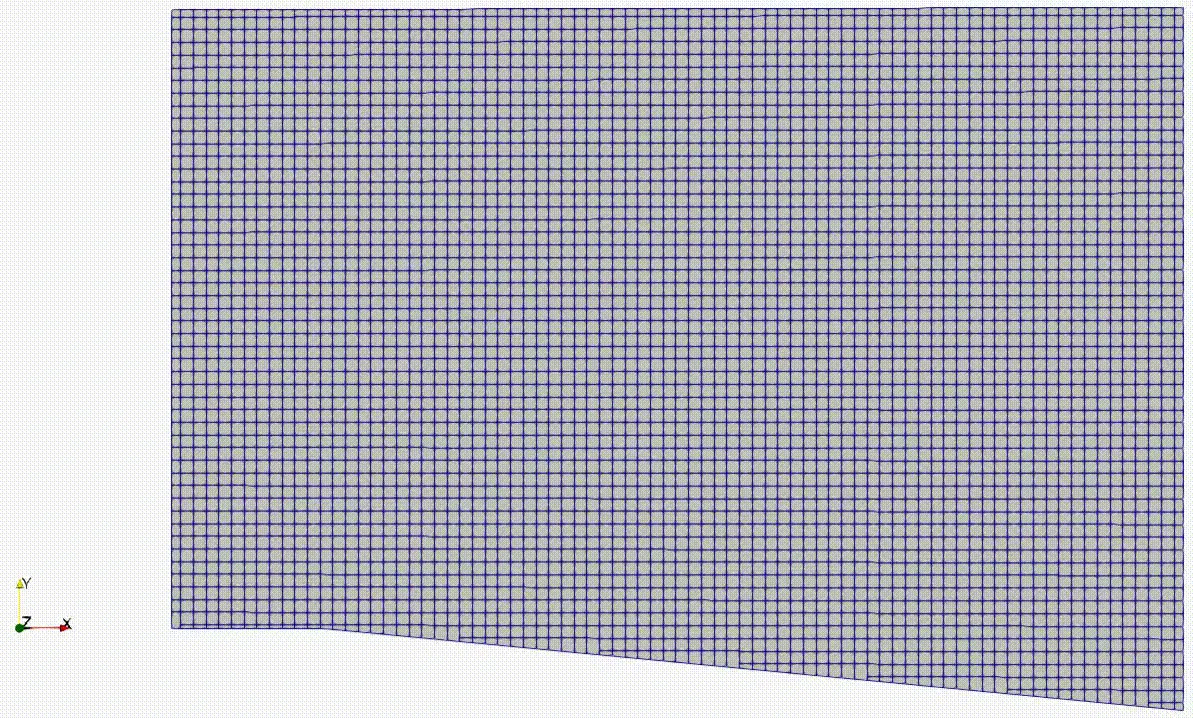
Fig. 5: Mesh 1 (two-dimensional sliced view)
Mesh 2:
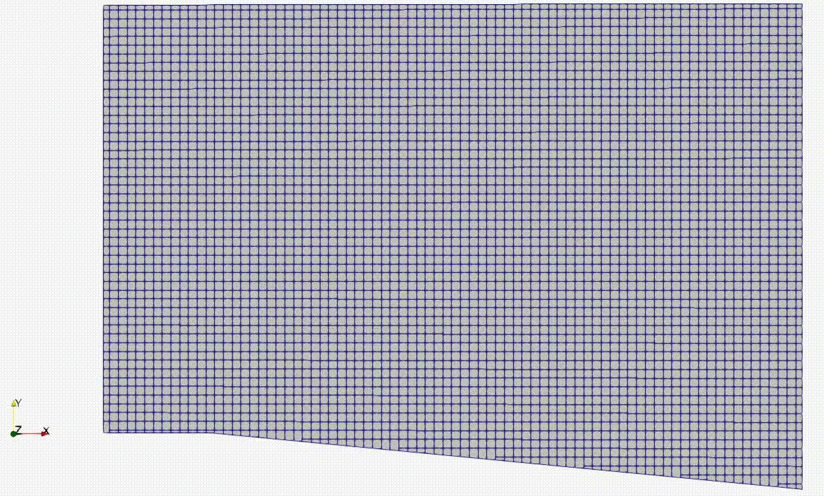
Fig. 6: Mesh 2 (two-dimensional sliced view)
Mesh 3:
Fig. 7: Mesh 3 (two-dimensional sliced view)
Mesh 4:
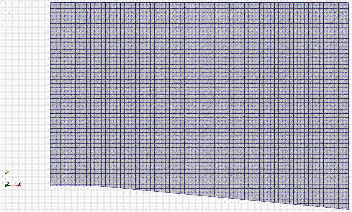
Fig. 8: Mesh 4 (two-dimensional sliced view)
Mesh 5:
Fig. 9: Mesh 5 (two-dimensional sliced view)
| Mesh | Mach Number (`M_2`) | % var | Static Pressure (`p_2`) (`N/m^2`) | % var | Density (`rho_2`) (`(kg)/m^3`) | % var | Temperature (`T_2`) (`K`) | % var | Velocity (u) (`m/s`) | % var | Velocity (v) (`m/s`) | % var |
| Baseline | 2.1891 | -- | 74285.3 | -- | 0.9838 | -- | 262.0796 | -- | 709.5199 | -- | -65.6608 | -- |
| 1 | 2.1906 | 0.0685 | 74169.4 | -0.1560 | 0.9827 | -0.1118 | 261.959 | -0.046 | 709.837 | 0.0447 | -65.659 | -0.0027 |
| 2 | 2.1923 | 0.0776 | 74016.7 | -0.2063 | 0.9814 | -0.1323 | 261.779 | -0.0687 | 710.089 | 0.0355 | -66.251 | 0.9016 |
| 3 | 2.1921 | -0.0091 | 74018.8 | 0.0028 | 0.9814 | 0 | 261.779 | 0 | 710.038 | -0.0072 | -66.292 | 0.0619 |
Table 10: Percentage variation in values of flow-field parameters for different mesh configurations whose maximum embed level was constant
| Mesh | Mach Number (`M_2`) | % var | Static Pressure (`p_2`) (`N/m^2`) | % var | Density (`rho_2`) (`(kg)/m^3`) | % var | Temperature (`T_2`) (`K`) | % var | Velocity (u) (`m/s`) | % var | Velocity (v) (`m/s`) | % var |
| Baseline | 2.1891 | -- | 74285.3 | -- | 0.9838 | -- | 262.0796 | -- | 709.5199 | -- | -65.6608 | -- |
| 2 | 2.1923 | 0.1462 | 74016.7 | -0.3616 | 0.9814 | -0.2439 | 261.779 | -0.1147 | 710.089 | 0.0802 | -66.251 | 0.8989 |
| 4 | 2.1925 | 0.00912 | 73988 | -0.0388 | 0.9812 | -0.0204 | 261.74 | -0.0149 | 710.14 | 0.00718 | -66.32 | 0.1041 |
| 5 | 2.1928 | 0.0137 | 73970 | -0.0243 | 0.9810 | -0.0204 | 261.72 | -0.0076 | 710.18 | 0.00563 | -66.39 | 0.1055 |
Table 11: Percentage variation in values of flow-field parameters for different mesh configurations whose SGS-based temperature values were constant
| Flow-field parameters | Exact, Analytical Solution | Baseline Mesh | % error | Mesh 1 | % error | Mesh 2 | % error | Mesh 3 | % error | Mesh 4 | % error | Mesh 5 | % error |
| Mach Number (`M_2`) | 2.2 | 2.1891 | -0.4954 | 2.1906 | -0.4273 | 2.1923 | -0.35 | 2.1921 | -0.3591 | 2.1925 | -0.3409 | 2.1928 | -0.327 |
| Static Pressure (`p_2`) (`N/m^2`) | 73900 | 74285.3 | 0.5214 | 74169.4 | 0.3645 | 74016.7 | 0.1579 | 74018.8 | 0.1607 | 73988 | 0.1191 | 73970 | 0.0947 |
| Density (`rho_2`) (`(kg)/m^3`) | 0.984 | 0.9838 | -0.020 | 0.9827 | -0.1321 | 0.9814 | -0.2642 | 0.9814 | -0.2642 | 0.9812 | -0.2845 | 0.9810 | -0.3049 |
| Temperature (`T_2`) (`K`) | 262 | 262.0796 | 0.0304 | 261.959 | -0.016 | 261.779 | -0.0843 | 261.779 | -0.0843 | 261.74 | -0.0992 | 261.72 | -0.1069 |
| Velocity (u) (`m/s`) | 710 | 709.5199 | -0.0676 | 709.837 | -0.0229 | 710.089 | 0.0125 | 710.038 | 0.005 | 710.14 | 0.0197 | 710.18 | 0.0253 |
| Velocity (v) (`m/s`) | -66.5 | -65.6608 | -1.2619 | -65.659 | -1.2647 | -66.251 | -0.3744 | -66.292 | -0.3128 | -66.32 | -0.2707 | -66.39 | -0.165 |
Table 12: Percentage error comparison between predicted values of flow-field parameters for different mesh configurations and exact, analytical solutions (Data highlighted in bold indicates the least value of percentage error for that parameter)
Time statistics and Mesh quality attributes for the different mesh configurations:
|
Mesh |
Total Cells |
Run Time [s] |
Max Aspect Ratio |
Max Skewness |
Max Non-Orthogonality |
|
Baseline |
4179 |
183.0637 | 3.32889 | 1.17578e-38 | 30.0143 |
|
1 |
4191 | 161.6574 |
3.32889 |
1.17578e-38 |
31.0416 |
|
2 |
12153 | 455.8249 |
3.32889 |
1.17578e-38 |
30.9242 |
|
3 |
17858 | 797.3621 |
3.32889 |
1.17578e-38 |
35.4901 |
|
4 |
19564 | 784.8834 | 3.32889 | 1.17578e-38 | 33.6901 |
|
5 |
29675 | 1252.0538 | 3.32889 | 1.17578e-38 | 67.9033 |
Table 13: Time statistics and Mesh quality attributes depicting the maximum values of aspect ratio, skewness and non-orthogonality for different mesh configurations of the domain consisting of supersonic flow through a centered expansion wave
From the meshing statistics in Table 10 and Table 11, it can be seen that across a range of mesh configurations for supersonic flow through a centered expansion wave, mesh number 2 (or mesh 2) with 12153 cells indicates an overall minimum percentage variation in values for almost all of its flow-field parameters except for static pressure (`p_2`), Density (`rho_2`) and Temperature (`T_2`) in the case of mesh configurations with different maximum embed levels i.e., mesh 4 and mesh 5, wherein, the variations reported in those quantities required a significant increase in computational resources, as seen in Table 13, however, without affecting the corresponding predictions made previously i.e., using mesh 2, significantly. The % var is calculated as the ratio of the difference of the predicted values in two consecutive meshes to the predicted value of the previous mesh e.g., ((Mach number for Mesh 2 - Mach number for Mesh 1)/Mach number for Mesh 1). Similarly, mesh number 5 (or mesh 5) with 29675 cells represents the least value of percentage error in prediction for most of the different flow-field parameters at the outlet (averaged quantities in the region occupied by the trailing edge of the expansion wave and the wall boundary surface along the expansion corner) when compared against the exact, analytical solution, as seen in Table 12, however, a simultaneous closer look at Table 13 reveals that from Mesh 2, the difference in percentage error does not drastically change as much as the resultant increase in computational resources i.e., decreasing the sub-grid criterion or increasing the maximum embedding level does not significantly alter the prediction of most of the flow-field parameters in comparison to a large increase in number of cells created based on the AMR requirements and the subsequent rise in computational time. Therefore, a mesh independent result can be said to have been achieved with the Mesh 2 configuration and the same to be validated against the exact, analytical solution as the percentage difference in accuracy between them is under 0.5% for all of the previously mentioned flow-field parameters. It should be noted that the sub-grid criterion value for the given numerical simulation can be deduced with the help of (Eq. 1), (Eq. 2) and (Eq. 4), however, this method is unfeasible as the number of Mach waves (or lines) originating from the given expansion corner are essentially infinite and therefore the value listed in Table 9 may be considered a reasonable approximation such that the resolved flow-field in the expansion fan region provides a sufficiently clear visualisation of temperature as well as the remaining parameters with accuracy especially downstream of the expansion wave for the mesh independent result to be quite reliable based on its configuration. Additionally, mesh quality attributes of all the different meshes prepared in Table 13 indicates that they lie in the range of acceptable value for skewness, as previously stated in Table 1, remains constant for aspect ratio but deteriorates for non-orthogonality with increase in maximum embedding level or decrease in sub-grid criterion as the change in the cell sizes became more discontinuous owing to the impact on the resolution due to differences between the actual field and resolved field based on the computation of temperature gradients especially in the region of the expansion fan and to a certain extent along the slip wall boundary surfaces. Results in Section 3 dealing with visualisation of flow-field parameters using field plots will only be referred with regards to the mesh independent solution i.e., Mesh 2.
2.6 Convergence Level
In the given numerical analysis, a steady-state simulation was performed using a Density-based solver, to account for the compressibility effects, of type modified Pressure Implicit with Splitting of Operator (PISO) which is an iterative pressure-velocity coupling algorithm involving a predictor step for predicting solution of the momentum equation from which a pressure equation is obtained and solved whose correction is then consequently reapplied to the momentum equation such that this process continues until the desired level of accuracy is achieved. At the end of the momentum predictor and first corrector step, remaining transport equations are solved in series. In other words, momentum and pressure are solved at the first PISO iteration which enables calculation for velocity terms required by other transport equations and at the end of each iteration in the PISO loop, convergence criterion is checked for which in the case of compressible flow requires the density correction error term to be less than the value of PISO tolerance which remains unchanged for the given numerical simulation at its default value of 1e-03. The selection of solver types for the different equations within 'Solver parameter [Steady-state]' sub-option in the 'Simulation Parameters' settings under the 'Case Setup' tree included assigning SOR to Momentum, Density, Energy, and 'CONVERGE BiCGSTAB' to the Pressure equation. The SOR solver type is a generally preferred algorithm owing to its advantage in being computationally less expensive than the different forms of biconjugate gradient stabilized (BiCGSTAB) algorithms or HYBRID (wherever applicable) except for the pressure equation unless the number of iterations for this equation (pressure) is less than 15 on average making it suitable for cases that contains a compressible flow with smaller value of time-steps. However, for the concerned numerical simulation, the default 'CONVERGE BiCGSTAB' algorithm was retained as it was difficult to estimate whether or not the pressure equation would always result in less than 15 iterations on average for different mesh configurations. BiCGSTAB algorithm works best in scenarios for which simulations approach convergence at a slower rate making it more suitable for multiphase flow simulations like volume of fluid (VOF). Also, as previously mentioned in Section 2.3.2 Boundary Conditions and Monitoring Points, the behaviour of mach number, density, static pressure and temperature at the outlet were being monitored as the quantities of interest to observe the variation in their values over successive cycles. The solver types, convergence tolerance limits, and minimum and maximum iterations defined for the equations corresponding to the default physical model and the monitor variable plots corresponding to the different mesh configurations are shown in the table and figures below:
|
Equations |
Solver Type |
Convergence Tolerance |
Minimum Iterations |
Maximum Iterations |
Preconditioner |
|
Momentum |
SOR |
1e-05 |
2 |
50 |
None |
|
Pressure |
CONVERGE BiCGSTAB |
1e-08 |
2 |
300 |
None |
|
Density |
SOR |
1e-04 |
2 |
20 |
None |
|
Energy |
SOR |
1e-04 |
2 |
20 |
None |
Table 14: Solver Types, Convergence Tolerance Values, Minimum and Maximum Iterations and Preconditioners of the different equations used in the default physical model
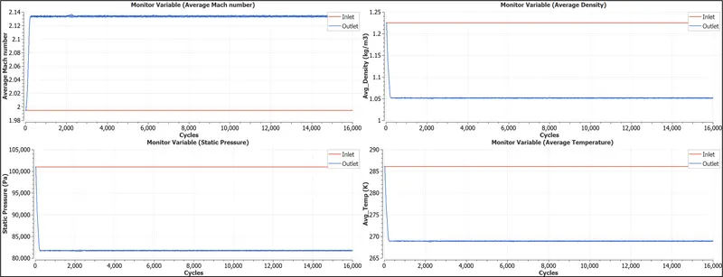
Fig. 10: Plots of monitor variables mach number, average density, static pressure and average temperature for steady-state simulation of supersonic flow through a centered expansion wave using the baseline mesh
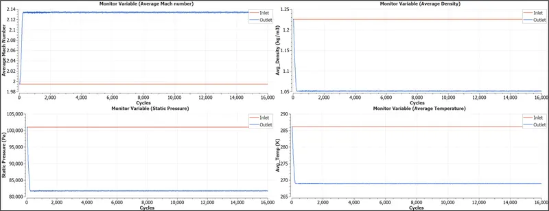 Fig. 11: Plots of monitor variables mach number, average density, static pressure and average temperature for steady-state simulation of supersonic flow through a centered expansion wave using mesh 1
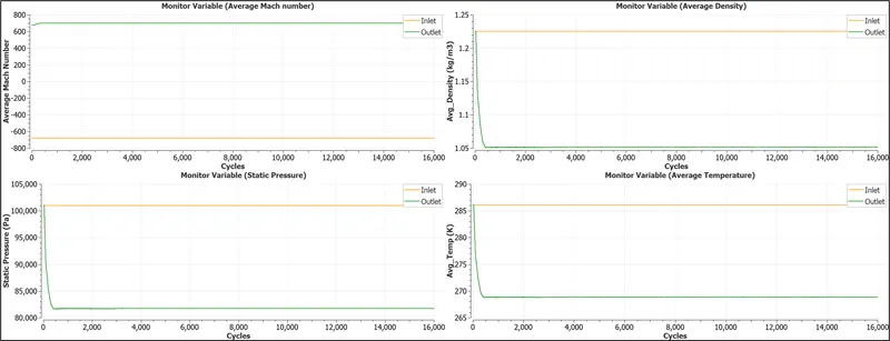
Fig. 12: Plots of monitor variables mach number, average density, static pressure and average temperature for steady-state simulation of supersonic flow through a centered expansion wave using mesh 2
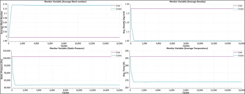
Fig. 13: Plots of monitor variables mach number, average density, static pressure and average temperature for steady-state simulation of supersonic flow through a centered expansion wave using mesh 3
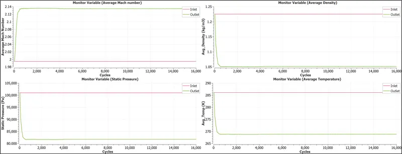
Fig. 14: Plots of monitor variables mach number, average density, static pressure and average temperature for steady-state simulation of supersonic flow through a centered expansion wave using mesh 4
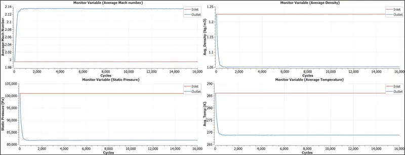
Fig. 15: Plots of monitor variables mach number, average density, static pressure and average temperature for steady-state simulation of supersonic flow through a centered expansion wave using mesh 5
From Fig. 10 and Fig. 11, it can be observed that the monitor variables oscillate with varying degree of fluctuations that appear to be repetitive at their respective frequencies over a large number of cycles indicating that the solution can be deemed to have achieved convergence as opposed to a highly stable output in the same monitor variables noticed in Fig. 12, Fig. 13, Fig. 14 and Fig. 15, well before they reach the end of total number of cycles specified in the 'End time' parameter under the 'General' tab of 'Simulation Parameters' settings under the 'Case Setup' tree as 25000, also indicating that a steady-state solution was obtained.
3. Results
3.1 Velocity magnitude, mach number, density, static pressure and temperature values using field plots
Fig. 16 to Fig. 20 below shows the velocity magnitude, mach number, density, static pressure and temperature values for mesh independent result, mesh 2, across the domain consisting of supersonic air flow movement through a centered expansion wave in two-dimensional space using field plots at the slice region created by orienting the plane normal to the flow direction as was specified in Section 2.4 Post-Processing. It can be observed that the expansion fan region created due to the expansion corner is continuous and the values also vary in a smooth manner across it with the flow downstream of the expansion wave accelerating while the static flow properties viz., static pressure, density and temperature, all but decreasing accordingly.
Fig. 16: Velocity Magnitude field plot across the domain for mesh 2 in two-dimensional space
Fig. 17: Mach number field plot across the domain for mesh 2 in two-dimensional space
Fig. 18: Density field plot across the domain for mesh 2 in two-dimensional space
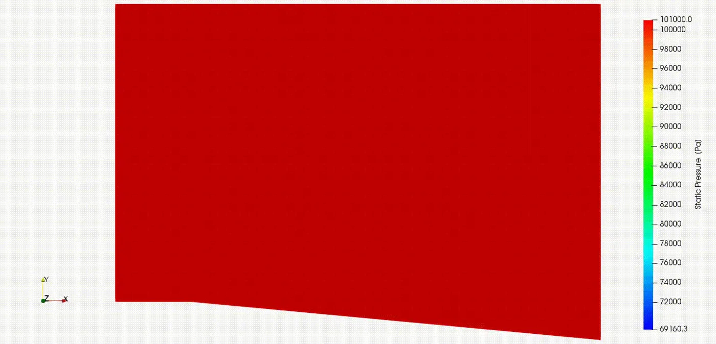
Fig. 19: Static pressure field plot across the domain for mesh 2 in two-dimensional space
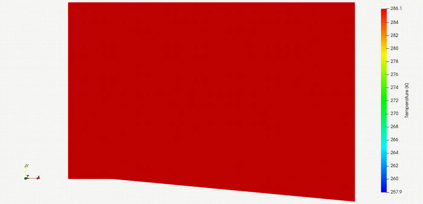
Fig. 20: Temperature field plot across the domain for mesh 2 in two-dimensional space
3.2 Velocity magnitude and Velocity (x-component), mach number, density, static pressure and temperature values using line plots
Fig. 21 and Fig. 23 below shows the comparison between the flow-field properties of supersonic flow through a centered expansion wave predicted by different mesh configurations and the exact, analytical solution for the given setup at x-coordinate position of 12.928m wherein with every subsequent mesh refinement either by decreasing the temperature dependent sub-grid criterion or increasing the maximum embedding level, the differences in the direction of maximum gradient change i.e., y-axis orientation, especially at the location close to the wall boundary surface along the expansion corner becoming smaller as opposed to initial observations made with the baseline mesh. Similarly, the x-component of velocity, `u`, profile plots at x-coordinate positions of 16.17m, 32.21m and 48.99m also highlights a remarkable improvement in agreement against its counterpart exact, analytical solution profiles using SGS-based AMR of temperature dependent sub-grid criterion combined with appropriate maximum embedding level featuring the importance of the implemented meshing approach in this numerical simulation which was to effectively refine the mesh in the region where maximum change in gradients was most likely to occur in order to better capture the underlying physics without drastically affecting the mesh quality while retaining the remaining area with the base grid size settings.
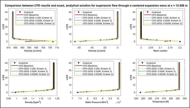
Fig. 21: Comparison between CFD results using different mesh configurations (varying SGS, constant maximum embedding level) and exact, analytical solution of different flow properties for supersonic flow through a centered expansion wave at x = 12.928m from inlet boundary surface
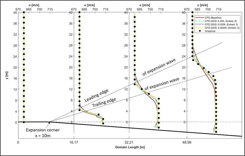
Fig. 22: Comparison between CFD results using different mesh configurations (varying SGS, constant maximum embedding level) and exact, analytical solution of u [m/s] for supersonic flow through a centered expansion wave at x = 0m, 16.17m, 32.21m and 48.99m from inlet boundary surface (Adapted from [1] based on current numerical simulation]
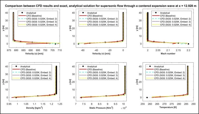
Fig. 23: Comparison between CFD results using different mesh configurations (varying maximum embedding level, constant SGS) and exact, analytical solution of different flow properties for supersonic flow through a centered expansion wave at x = 12.928m from inlet boundary surface
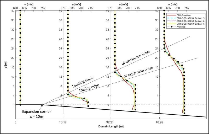
Fig. 24: Comparison between CFD results using different mesh configurations (varying maximum embedding level, constant SGS) and exact, analytical solution of u [m/s] for supersonic flow through a centered expansion wave at x = 0m, 16.17m, 32.21m and 48.99m from inlet boundary surface (Adapted from [1] based on current numerical simulation]
4. Discussion
Air, containing a mixture of two major contributing gas species `O_2` and `N_2` by mass fraction, enters at the inlet of the given domain consisting of a convex corner, with regards to the angle created with the upstream wall surface, at a position of 10m along the bottom wall from the inlet as supersonic flow. The flow remains essentially parallel and unaffected with respect to the walls bounding it which are of the type "slip" condition such that the effects of viscosity are negligible or quite simply the flow can be described as inviscid which is in line with the modelling considerations made for this numerical study. As the supersonic flow approaches the convex corner, a continuous expanding region gets created, also called as an expansion fan, which are composed of infinite Mach waves that are also known as the Prandtl-Meyer expansion waves, after the two authors whose initial contributions paved the way to understanding these phenomena in greater detail. The characteristic behaviour of the Prandtl-Meyer expansion waves is that the change in flow properties does not occur abruptly but rather gradually with the expansion defined at an infinitesimal rate governed by the presence of each individual Mach wave in its infinite total. Also, a single Mach wave in the expansion fan region represents a line of constant properties thereby making the flow in this zone to be isentropic in nature. The supersonic flow beyond the expansion wave region created by the convex corner accelerates while its other static properties such as pressure, density and temperature decreases.
5. Conclusion
The numerical analysis for two-dimensional, steady-state simulations of supersonic flow moving over a surface consisting of a convex corner using the default physical model in Converge Studio v3.0 and executed using the Cygwin64 terminal was well understood. It was realised that implementing a SGS-based AMR of temperature dependent sub-grid criterion for the given numerical study greatly improved the visualisation of the expansion wave region created by the convex corner while retaining the base grid size settings everywhere else which greatly assisted in keeping the total cell count lower, as well as lead to an overall better agreement with the exact, analytical solution.
References
[1] John D. Anderson, Jr., (1995). COMPUTATIONAL FLUID DYNAMICS: The Basics with Applications (Eds.), Numerical Solution of a Two-Dimensional Supersonic Flow: Prandtl-Meyer Expansion Wave (2nd ed., pp. 374–415). McGraw-Hill.
[2] CONVERGE 3.0 Manual. © 2020 Convergent Science. All rights reserved. July 15, 2020.