Week 4.2: Project Transient simulation of flow over a throttle body
1. Introduction
A throttle body valve fitted within a pipe works principally the same as a butterfly valve which is to regulate the movement of water across the confined pipe boundaries by rotating a disc typically mounted on a shaft whose motion can be controlled either manually with the help of a hand lever or gear, or automatically using electric, pneumatic or hydraulic actuation methods. The advantages of a throttle body (same as a butterfly valve) include ease in operation as a result of attaining fully-opened or closed position by only performing a 90° turn, also known as quarter-turn based on its value with respect to circular motion, relatively cheaper construction due to less material requirements, less space demands, and more importantly and usually offering great reliability in terms of service life because of less wear and tear and consequently improved maintenance.
The aim of this challenge was to perform a three-dimensional, transient state simulation using Realizable k-`epsilon` (RKE) turbulence model for an elbow-shaped pipe domain consisting of a rotating throttle body utilising the mesh independent result from the steady-state simulations in the previous challenge. The analysis involved quantitative measurements such as impact on mass flow rate with regards to throttle body positions at different time intervals as well as qualitative aspects including variations in velocity magnitude profiles and pressure drop values at the inlet and outlet regions of the domain at different time intervals, and identification of separation and recirculation regions.
2. Method
The typical approach adopted to performing numerical simulations in CONVERGE CFD involves the following steps:
- Creating a new folder dedicated to running the concerned project inside a user-preferred directory.
- Setting up the relevant case file(s) in Converge Studio v3.0 that involves creation of the fluid volume domain, setting up the required application type, choosing material and its state (gas, liquid, parcel or solid) for which simulation is to be performed along with the requisite properties, defining simulation parameters such as solver types, run time variables, and convergence tolerances, defining region(s), boundary conditions and initial conditions, specifying the physical models whose equations are intended to be solved, determining and allocating the base grid size values as well as any other refinements, and lastly selecting the variables for post-processing at the required time intervals along with any hidden parameters or UDF selection as part of advanced parameters.
- Saving the case file(s) and exporting the input files into the folder created for running the concerned project which typically includes 'boundary.in' for the various boundary conditions, 'material_state.dat' where material_state points to either 'gas', 'liquid', 'parcel' or 'solid', 'initialize.in' specifying initial conditions, 'inputs.in' defining the various input conditions and file writing intervals, 'turbulence.in' containing information about the turbulence model selected and its associated constants, 'post.in' for the different post-processing variables, 'solver.in' describing the solver chosen and its equations, and 'surface.dat' containing datasets about the surface while other input files with respect to the state of the material, thermal properties and species may also be part of the exporting process and should be ensured that they are selected for the simulation to run.
- Running the simulation in a Cygwin64 terminal window.
- Post-converting 3D output data by navigating to the output folder created within the same project folder during the simulation run or from the 'Post-Processing 3D' button in Converge Studio v3.0.
The simulation run and post-converting processes were executed using Linux-type commands in a Cygwin64 terminal window as shown below:
i) Change directory to the project containing the relevant case file(s):
cd "PATH_TO_CONCERNED_PROJECT_FOLDER"
ii) Confirm the contents of the project for the exported input files:
ls
iii) Performing simulation run with the converge executable application on multiple processors (in this case, 4) using mpiexec executable file in the background (by adding ampersand operator) along with posting output into a logfile:
mpiexec.exe -n 4 converge.exe restricted </dev/null> logfile &
iv) Checking for simulation status with regards to completion or errors:
tail logfile
v) Post-converting the 3D output data files using the 'post_convert_30_msmpi_64' utility on multiple processors (in this case, 4) using mpiexec executable file from within the output folder of the project containing the exported input files:
cd output
mpiexec.exe -n 4 post_convert_30_msmpi_64
2.1 Modelling
The computational domain for transient state simulation of air flow movement through an elbow-shaped pipe with a rotating throttle body was constructed using the same model from the previous challenge for the steady-state simulations in Converge Studio v3.0 with similar boundary surfaces i.e., Inlet, Outlet, Elbow Pipe Walls and Throttle Body as illustrated in Fig. 1 with the difference being the application of rotary motion to the throttle body which was incorporated by assigning a moving surface movement about its rotation axis upto an angle of 25°, more of which has been discussed in Section 2.2.1 Boundary Conditions.
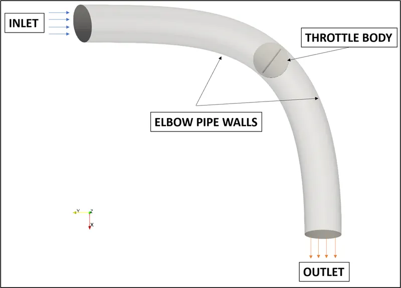
Fig. 1: Fluid Volume Model and Boundary Conditions regions in three-dimensional space
2.2 CFD Simulation Setup, Boundary Conditions and Determination of transient parameters
The transient simulation on mesh independent result (Mesh 2) from the steady-state simulations in the previous challenge was performed using the Reynolds Averaged Navier-Stokes (RANS) models, in this case, the k-`epsilon` turbulence models. The use of k-`epsilon` turbulence models and more specifically the RKE turbulence model is attributed to the fact that the Reynolds number, based on the given flow conditions, lies in the turbulence flow region as well as representing high Reynolds number attached flows for which the solution variables, like the velocity profile, was modelled for the log-law layer using the standard wall function approach such that the first grid cell would lie in the range of 30<`y^+`<300 in order to yield satisfactory results. A brief description about the RKE turbulence model and its setup were already mentioned for the steady-state simulations in the previous challenge.
2.2.1 Boundary Conditions
The different boundary conditions for transient simulation of air flow movement through an elbow-shaped pipe with a rotating throttle body is described in the following table:
|
Names |
Inlet |
Throttle_Body_wall |
Elbow_pipe_walls |
Outlet |
|
Type |
INFLOW |
WALL |
WALL |
OUTFLOW |
|
Pressure Boundary Condition |
Specified Value (DI), Total pressure |
-- |
-- |
Specified Value (DI) |
|
Pressure Magnitude (Pa) |
150000 |
-- |
-- |
100000 |
|
Velocity Boundary Condition |
Zero normal gradient (NE) |
-- |
-- |
Zero normal gradient (NE) |
|
Temperature Boundary Condition |
Specified Value (DI) |
Specified Value (DI) |
Specified Value (DI) |
-- |
|
Temperature Backflow |
-- |
-- |
-- |
Specified Value (DI) |
|
Temperature Magnitude (K) |
300 |
300 |
300 |
300 |
|
Species Boundary Condition |
Specified Value (DI) |
-- |
-- |
Specified Value (DI) |
|
Species Name: `O_2` |
0.23 |
-- |
-- |
0.23 |
|
Species Name: `N_2` |
0.77 |
-- |
-- |
0.77 |
|
Wall motion type |
-- |
Rotating |
Stationary |
-- |
|
Surface Movement |
-- |
Moving, Law of wall |
Fixed, Law of wall |
-- |
|
Turbulent Kinetic Energy (tke) |
Intensity, 0.033 fraction [1] |
Zero normal gradient (NE) |
Zero normal gradient (NE) |
-- |
|
Turbulent Dissipation (eps) |
Length scale, 0.001202m [2] |
Wall model |
Wall model |
-- |
|
Turbulent Kinetic Energy (tke) Backflow |
-- |
-- |
-- |
Intensity, 0.033 fraction [1] |
|
Turbulent Dissipation (eps) Backflow |
-- |
-- |
-- |
Length scale,0.001202m [2] |
|
Near wall treatment |
-- |
Standard wall function |
Standard wall function |
-- |
|
Law of wall roughness parameters; Absolute roughness |
-- |
0.0m |
0.0m |
-- |
|
Law of wall roughness parameters; Roughness constant |
-- |
0.5 |
0.5 |
-- |
Table 1: Boundary Conditions for the elbow-shaped pipe domain consisting of a rotating throttle body defined using the 'Boundary' sub-option of the 'Boundary Conditions' under the 'Case Setup' tree
For the given transient state problem, the simulation was chosen as 'Gas simulation', similar to the steady-state simulation performed on the same model, with material selected as 'Air' and 'Species (not in mech.dat)' option enabled to utilise the mass fraction values of `O_2` and `N_2` as they represent the major constituting species in air by mass fraction. Additionally, the Redlich-Kwong (RK) cubic equation of state was set to in the 'Equation of state' drop-down menu with its default values of critical temperature (`T_c`) and critical pressure (`p_c`) retained at '133.0 K' and '3770000.0 Pa' respectively to describe the coupling relationship between the different state variables such as density and physical conditions such as pressure and temperature depicting the state of matter with the real gas properties behaving as a function of temperature which was again set to as the default option in the 'Gas simulation' window while the values of 'Turbulent Prandtl number' and 'Turbulent Schmidt number' were left unchanged at their default values of 0.9 and 0.78 respectively. The rotation of the throttle body was specified by defining the rotation center and rotation axis with the help of 'Direction' option available as a subset when the 'Measure' button was clicked on under the 'Geometry' dock and then describing the following profile information:
| Second | Angle |
| 0.0 | 0.0 |
| 0.002 | 25.0 |
| 0.004 | 25.0 |
| 0.008 | 0.0 |
Table 2: Profile information for rotation of the throttle body
2.2.2 Determination of transient parameters
The setup of simulation run time and time-step for the given numerical problem was defined such that the 'Start time' in the 'Simulation Time parameters' window under the 'Case Setup' tree was set to 0s while the 'End Time' in the same window depended on the domain length and the flow velocity, in the direction of flow, such that the fluid medium passed through it at least 10 flow through times so as to capture the different positions of the rotating throttle body while also tending to steady state conditions when the throttle body valve position remains unchanged. Therefore, 'End Time' was evaluated as:
`End \ Time = (L/U)*10`; where (Eq. 1)
`L` is the length of the pipe determined as 0.2091378m, and
`U` is the fluid flow velocity determined from the converged state values of mesh independent (Mesh 2) in the previous steady-state simulations challenge as 180.724m/s
From Eq. 1, we get value of 'End Time' approximately as 0.01157s. Time-step was decided based on the CFL number which is expressed below:
`CFL = (U*Delta t)/(Delta x)`; where (Eq. 2)
`Delta t` is time-step,
`Delta x` represents the smallest cell size, which in this case was determined as the smallest complete cell size in the laminar boundary layer thickness region surrounding the throttle body at fully-opened position resulting in a value of 0.000143746m.
In order to attain temporal accuracy and numerical stability, the CFL criteria was decided to be 1 and therefore, the value of time-step determined with this limiting value equated to 7.953e-7s. This value of time-step, however, reflects for a domain whose smallest cell size across it would consistently remain at the value of `Delta x`, as reported earlier, and at all times during the transient simulation which as a result of the cartesian cut-cell meshing approach cannot always be achieved and therefore, the time marching solution process or 'Time-step selection' chosen was of type 'Use variable time-step algorithm'. A variable time-step allows for internally calculated time-step that in turn depends on additional inputs including minimum and maximum time-step, maximum convection CFL, maximum diffusion CFL and maximum Mach CFL limit, among others, such that the resultant value determined based on the corresponding limiting conditions on the inputs would represent the maximum permissible time-step for the next iteration to be performed. The evaluation of initial, minimum and maximum time-steps as well as verification of moving boundary motion was performed using a 'No hydrodynamic solver (for testing setup only)' simulation which turned out to be a very useful feature as no transport equations were solved and thus improving utilisation of computational resources. The 'No hydrodynamic solver (for testing setup only)' simulation mode resulted in a successful run with initial, minimum and maximum time-steps values of 1e-11, 1e-11 and 1e-4 respectively. The maximum convection CFL was set to 1, as seen in (Eq. 2) above, and maximum Mach CFL limit estimated at 1.921 from (Eq. 3) [3] shown below, but the values were unaltered from their default settings for both maximum Mach CFL limit at 50 and maximum diffusion CFL of 2 (hand-calculation was not considered feasible as one of the variables reflected calculated cell value) to allow for larger time-step and subsequently faster run time.
`Mach \ CFL = (c*Delta t)/(Delta x)`; where (Eq. 3)
`c` is the speed of sound in gas determined from the following equation:
`c = sqrt((gamma*R*T)/(MW))`; where (Eq. 4)
`gamma` is the ratio of specific heats, equal to 1.4 [4],
`R` is the ideal gas constant, equal to 8.3144598 J/(mol.K) [5],
`T` is temperature of fluid at 300 K, and
`MW` is the molecular weight of air estimated to be 0.0289647 kg/mol [5]
2.2.3 Statistics of transient run for Mesh Independent Result (Mesh 2) from steady-state simulations
In this transient numerical simulation, the mesh independent result from steady-state simulations of the previous challenge was utilised for understanding the flow phenomena throughout the domain at different positions of the rotating throttle body, illustrated in Fig. 2, based on the profile information mentioned earlier in Table 2. It can be observed that the mesh especially at the boundary region surrounding the throttle body is constantly varying to accommodate cells based on the cartesian cut-cell approach as well as the fixed embedding definition with regards to the surface motion at different time-steps to ensure that the gradients at the wall are captured in the best possible way.
Mesh 2:
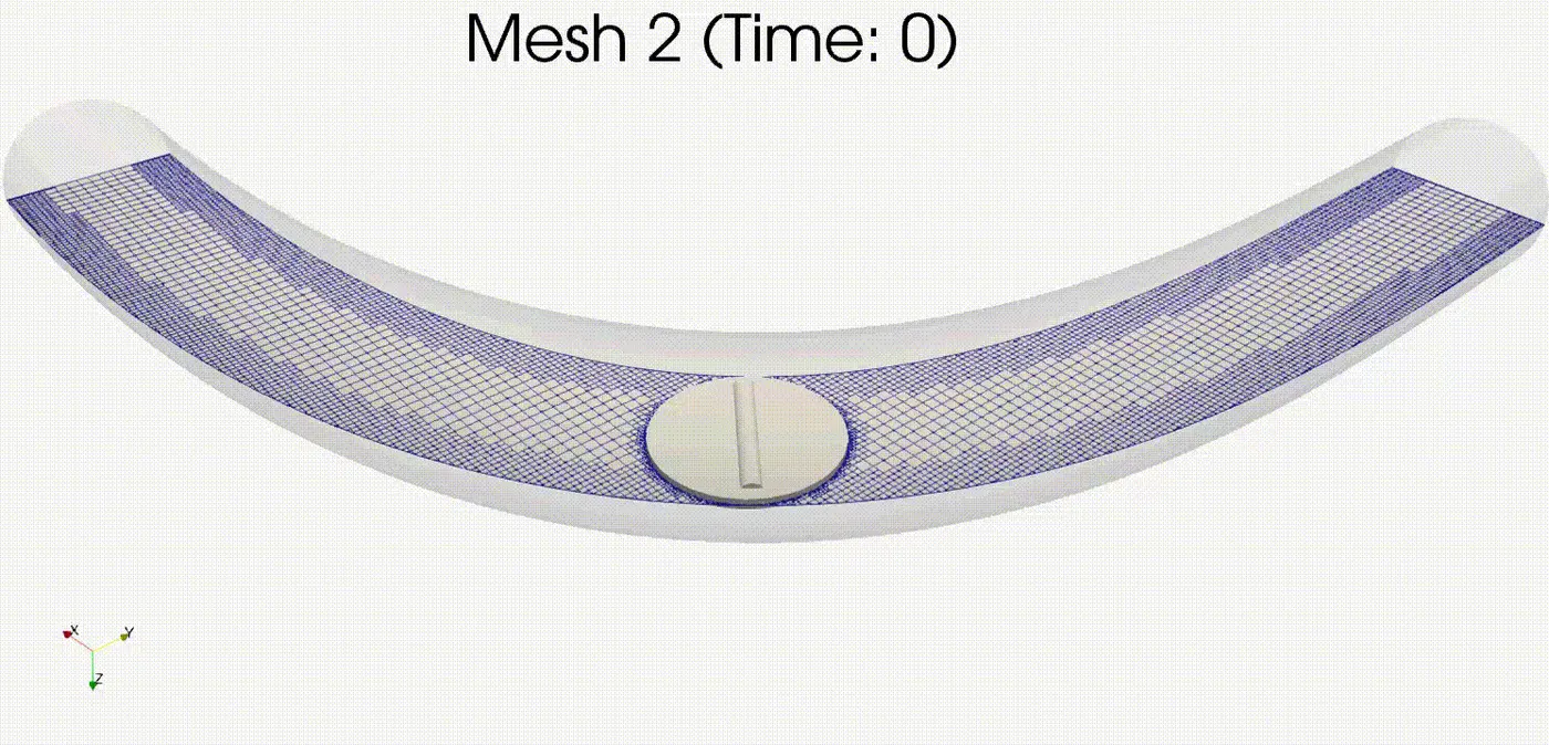
Fig. 2: Mesh 2 (three-dimensional sliced view)
Mesh and time statistics, peak velocity magnitude values near the outlet, and pressure drop across the domain for different meshes:
|
Mesh |
Cells |
Run Time [s] |
First Cell Height (`Delta_y`)[m] |
`y^+` (`y_P`) (Line 1) |
Peak Velocity Mag. [m/s] (Line 1) |
Pressure drop [Pa] |
|
2 |
241324 |
144627.9818 |
0.00033404 |
61.363 |
245.643 |
22423 |
Table 3: Mesh 2 time statistics, and peak velocity magnitude value at Line 1, pressure drop value across the domain, `y^+` at (`y_P`) at Line 1 at fully-opened throttle body position for the last time-step of the simulation run
Mesh quality attributes for Mesh 2:
|
Mesh |
Max Aspect Ratio |
Max Skewness |
Max Non-Orthogonality |
expansion ratio (first to 2nd layer of boundary cells) |
expansion ratio (last row of boundary cells to dy) |
|
2 |
3.4323 |
1.17578e-38 |
87.9037 |
1.721 |
~2 |
Table 4: Mesh 2 quality attributes depicting the maximum values of aspect ratio, skewness and non-orthogonality for the elbow-shaped pipe domain at fully-opened throttle body position for the last time-step of the simulation run
From the meshing statistics in Table 3, the difference between the prediction of peak velocity magnitude values at Line 1 and pressure drop values for mesh number 2 (or mesh 2) at transient state and steady state with same number of cells as 241324 is approximately equal to 10m/s and 1095 Pa respectively and as such the 'End Time' value for the transient setup would need to be further extended implying a significantly greater computational time. It can also be observed that the `y^+` value predicted at the first layer cell-centroid position is in the log-law region, however, with a similar notable difference between the initially calculated first cell height and the same computed by Converge as was reported in the steady-state simulations for the same model in the previous challenge.
2.3 Post-Processing
The variables of interest selected for the transient state simulation were exactly same as those of the steady-state simulations in the previous challenge which includes 'Density', 'Mesh Quality', 'Pressure', 'Temperature', 'Velocity', 'Region ID', 'Turbulent Kinetic Energy', 'Turbulent Viscosity', '`y^+`' , and 'Mass Fraction' for `O_2` and `N_2` species. Visualising the different flow variable quantities in two-dimensional space in ParaView required the creation of a slice of the given fluid domain by using the "Slice" tool in the 'Commons' toolbar typically located above the 'Pipeline Browser' window based on default layout settings and choosing 'Z Normal' under 'Plane Parameters' section to align the plane normal to the z-axis direction such that the entire domain was viewed in the direction of flow followed by unchecking the 'Show Plane' and 'Triangulate the slice' boxes for disabling the viewing of the plane borders and production of triangles in the output respectively. The velocity magnitude profiles near the outlet just after the analytically calculated fully-developed flow condition of the given domain for the fully-opened throttle body position was plotted using ParaView's in-built "plot over line" tool. The "plot over line" tool was accessed by clicking on 'Filters' present in the data analysis group, followed by entering the coordinates as seen in Table 5, and then clicking on the "Apply" button to view the said profile.
It was ensured that the last time-step of the simulation run was selected to view the velocity profile results. Additionally, velocity (U) and pressure (p) field plots were created in the form of 'Clip' and 'Slice' planes to view the development of the flow field characteristics across the fluid domain, and glyph based on stream tracers were added for identifying the high and low velocity regions. Legends, titles, and x and y labels were added for better understanding of the graphical representations.
|
Line 1 |
x |
y |
z |
|
Point 1 |
-0.00331697 |
0.01921 |
0.020174 |
|
Point 2 |
-0.00331697 |
0.0020424 |
0.020174 |
Table 5: Line Coordinates for viewing the velocity magnitude profiles
To save an animation plot of the different field plots, the option 'Save Animation' was accessed under the 'File' menu and clicked on followed by choosing the appropriate settings under the different sections such as 'Size and Scaling', 'Coloring', 'Compression Options' and 'Animation Options' to name a few, assigning an appropriate name to the animation file, in this case by the variable whose field plot is being indicated before clicking on the 'OK' button.
2.4 Convergence Level
In the given computational analysis, a transient state simulation using first-order implicit Euler time advancement scheme was performed to accommodate for larger time-steps while also being numerically stable along with a Density-based solver, to account for the compressibility effects, of type modified Pressure Implicit with Splitting of Operator (PISO) which is an iterative pressure-velocity coupling algorithm involving a predictor step for predicting solution of the momentum equation from which a pressure equation is obtained and solved whose correction is then consequently reapplied to the momentum equation such that this process continues until the desired level of accuracy is achieved. At the end of the momentum predictor and first corrector step, remaining transport equations are solved in series. In other words, momentum and pressure are solved at the first PISO iteration which enables calculation for velocity terms required by other transport equations and at the end of each iteration in the PISO loop, convergence criterion is checked for which in the case of compressible flow requires the density correction error term to be less than the value of PISO tolerance which remains unchanged for the given numerical simulation at its default value of 1e-03. The selection of solver types for the different equations within 'Solver parameters [Transient]' sub-option in the 'Simulation Parameters' settings under the 'Case Setup' tree included assigning SOR to Momentum, Pressure, Density, Energy, Turbulent Kinetic Energy (tke) and Turbulent dissipation rate (eps) equations. The SOR solver type is a generally preferred algorithm owing to its advantage in being computationally less expensive than the different forms of biconjugate gradient stabilized (BiCGSTAB) algorithms or HYBRID (wherever applicable). The solver types, convergence tolerance limits, and minimum and maximum iterations defined for the equations corresponding to the RKE turbulence model equations for the transient state simulation and the monitor variable plots are shown in the table and figures below:
|
Equations |
Solver Type |
Convergence Tolerance |
Minimum Iterations |
Maximum Iterations |
Preconditioner |
|
Momentum |
SOR |
1e-05 |
0 |
50 |
None |
|
Pressure |
SOR |
1e-08 |
2 |
500 |
None |
|
Density |
SOR |
1e-04 |
0 |
2 |
None |
|
Energy |
SOR |
1e-04 |
0 |
2 |
None |
|
Turbulent Kinetic Energy (tke) |
SOR (pre-defined) |
1e-03 |
2 |
50 |
None (pre-defined) |
|
Turbulent dissipation rate (eps) |
SOR (pre-defined) |
1e-03 |
2 |
50 |
None (pre-defined) |
Table 6: Solver Types, Convergence Tolerance Values, Minimum and Maximum Iterations and Preconditioners of the different equations used in the RKE turbulence model for transient state simulation
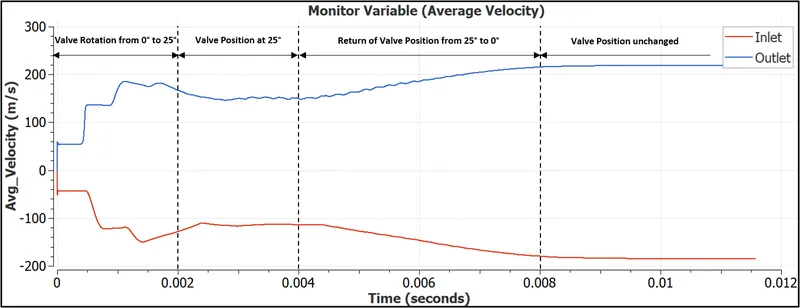
Fig. 3: Plot of monitor variable average velocity during transient state simulation using RKE turbulence model for mesh independent result (mesh 2) from the previous challenge
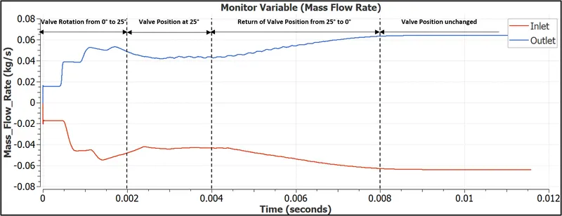 Fig. 4: Plot of monitor variable mass flow rate during transient state simulation using RKE turbulence model for mesh independent result (mesh 2) from the previous challenge
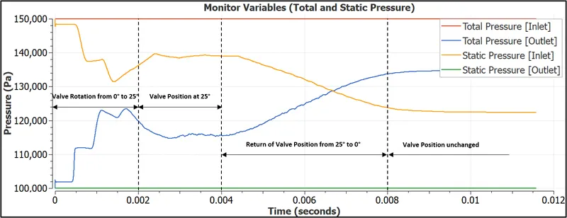
Fig. 5: Plot of monitor variables pressure (total and static) during transient state simulation using RKE turbulence model for mesh independent result (mesh 2) from the previous challenge
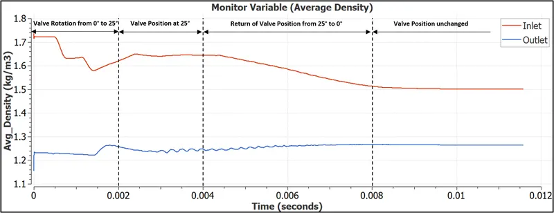
Fig. 6: Plot of monitor variable average density during transient state simulation using RKE turbulence model for mesh independent result (mesh 2) from the previous challenge
From Fig. 3, Fig. 4, Fig. 5 and Fig. 6, the variations in different monitor variables i.e., average velocity, mass flow rate, pressure (total and static) and average density respectively was observed at time intervals corresponding to throttle body rotation positions as described in its profile information in Table 2. As the valve rotates from 0° to 25° rotational position in the 0s to 0.002s time frame, the average velocity and mass flow rate at both the inlet and outlet boundaries, and total pressure at the outlet boundary initially rises with a slight drop towards the end while static pressure and average density at the inlet boundary decreases with a small but sudden sharp increase at their end before the same quantities assume less vigorously varying magnitudes when the valve remains stationary at the 25° rotation position from 0.002s to 0.004s followed by continuation of similar profiles as noticed in the 0s to 0.002s time frame only this time with more smoother gradients for 0.004s to 0.008s until eventually almost steady conditions are achieved towards the 'End Time' of the simulation when the valve position remains unchanged from 0.008s to 0.01157s. The volume-based conservation principles were followed, as observed from the plots in Fig. 3, Fig. 4, Fig. 5 and Fig. 6, because the mass flow rate at the inlet and outlet boundaries remained exactly the same indicating that the quantities velocity and density at the same two boundaries represented the actual flow conditions at the corresponding time intervals and more importantly, its inverse relationship with pressure indicated the direction of flow from a high pressure region, at the inlet boundary, to a low pressure region, at the outlet boundary. It should be noted that the values of different parameters and solver types highlighted in Table 6 were unaltered at the time of setup, or in other words based on default settings.
3. Results and Discussion
3.1 Velocity magnitude and pressure gradient values using field plots
Fig. 7 and Fig. 8 below shows the velocity magnitude and pressure gradients with respect to transient simulations performed on mesh independent result (Mesh 2), obtained from the steady-state simulations in the previous challenge, across the elbow-shaped pipe domain consisting of a rotating throttle body in three-dimensional space using "Clip " and two-dimensional views with "Slice" planes to display field plots as was mentioned in Section 2.3 Post-Processing. It can be observed that while initially a high pressure region is formed in front of the small upper section of the throttle body when the fluid strikes the same surface resulting in the velocity at that portion to become drastically low in value, the same high pressure region now shifts to occupy more of the throttle body's circular cross-sectional area as it gets projected to the incoming fluid during rotation from 0° to 25°. Also, the fluid on top of the throttle body surface in its immediate proximity typically indicates low velocity as a result of it being stuck onto it due to the boundary layer formation, except at the small curved region at the middle which usually consists of a shaft passing through it for allowing the rotary motion to happen in the first place, can be observed to undergo drastic changes in its values as the throttle body rotates from 0° to 25° such that the same surface transitions to a relatively low pressure region as a result of the rapidly accelerating flow over the moving zone because of the reduction in flow area between it and the elbow pipe walls.
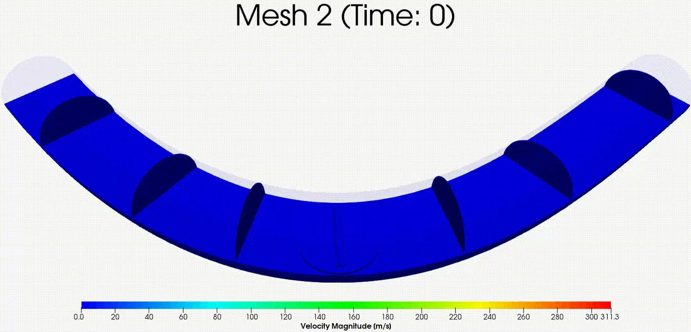
Fig. 7: Velocity Magnitude field plots using "Clip" and "Slice" planes across the domain for mesh 2 in three and two dimensional spaces
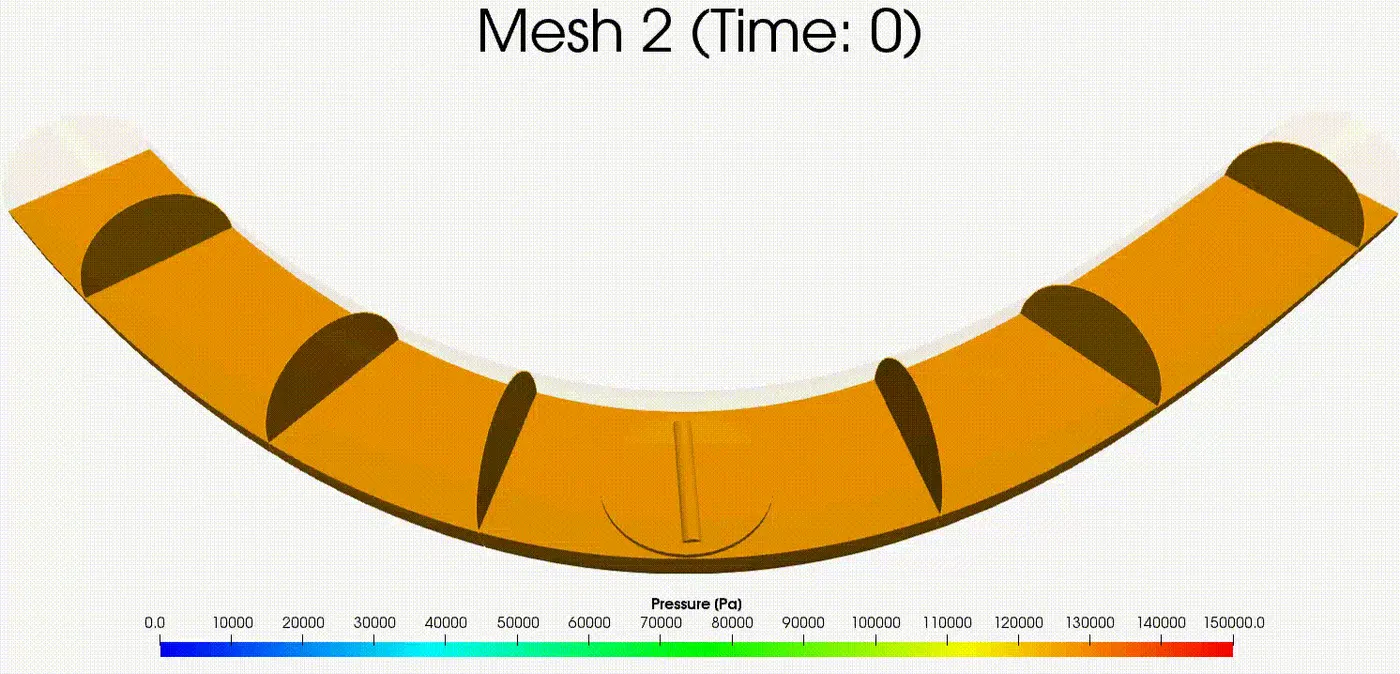
Fig. 8: Pressure field plots using "Clip" and "Slice" planes across the domain for mesh 2 in three and two dimensional spaces
3.2 Velocity magnitude values using line plots
The timewise variation in velocity magnitude profiles at Line 1 (near the domain outlet) for transient simulation on mesh independent result (Mesh 2) obtained from the steady-state simulations in the previous challenge can be viewed in Fig. 9 below. As it can be seen in the same figure, the position of the peak velocity magnitude switches from a smooth peak at the throttle body position of 0° rotation to a distinctively sharper peak at 25° with a much more adversely varying profile consisting of a sudden decline, or otherwise also known as a trough, before returning to the same shape for throttle body position at 0° rotation in a more gradual manner. The plot displaying the velocity profiles in Fig. 9 with respect to the text in the title changing as per the time interval could unfortunately not be created in ParaView due to software programming differences wherein the filters work on VTK windows platform as opposed to "plot over line" which was developed on Qt and as such the same was recreated in Matlab. It should also be noted that the end time in the same plot i.e., Fig. 9, represents 0.01157s, as mentioned in Section 2.2.2 Determination of transient parameters, and not 0.012s which is only an indication of arrival of the end state as the same value is based on a positive integer time advancing variable in a for loop.
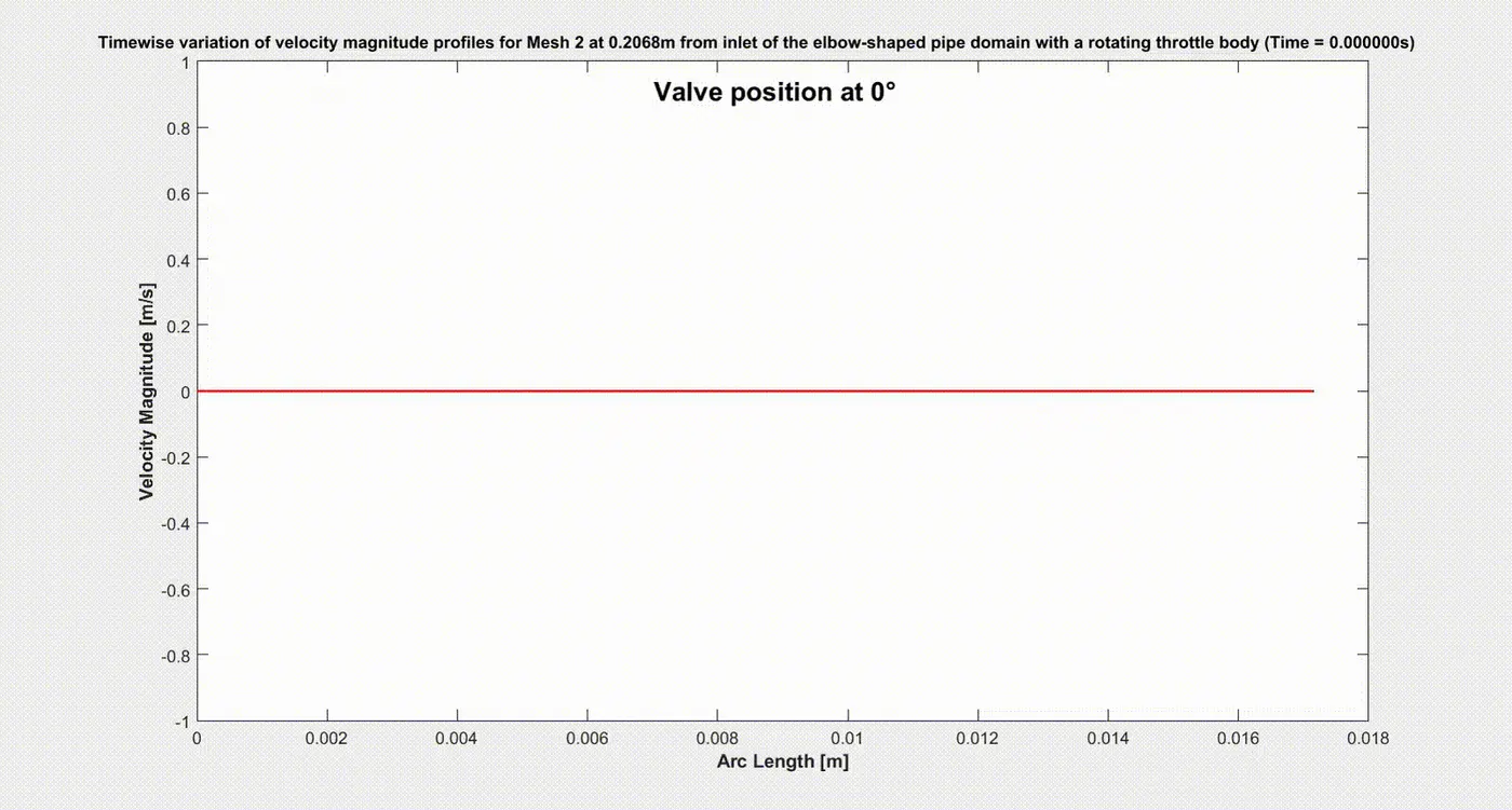
Fig. 9: Timewise variation of velocity profiles at 0.2068m from inlet of the elbow-shaped pipe domain with a rotating throttle body at Line 1
3.3 Separation and Recirculation regions
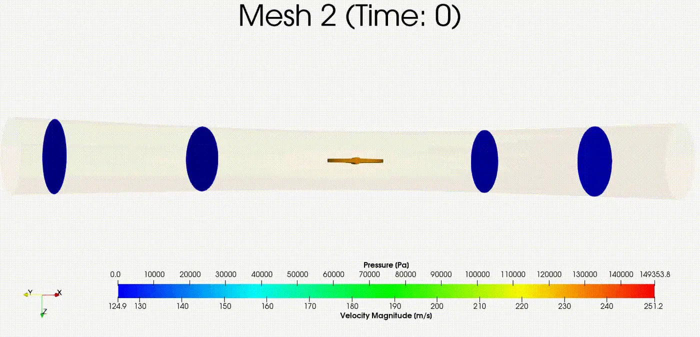
As observed in Fig. 10 a) and Fig. 10 b) below, velocity immediately vertically away, along the negative Z axis direction with respect to the throttle body, at 0° position was found to be gradually increasing due to the boundary layer formation on it while the presence of a curvature at the elbow bend causing pressure drop and making the flow in this region more prone to separation. During the rotation of the throttle body valve from 0° to 25°, the fluid flow separating in front of the throttle body now accelerates even more rapidly as spaces between the moving surface and the elbow pipe walls become narrower resulting into an erratically intense variation in the velocity magnitude with larger gradients also leading to formation of bigger swirling flows. A recirculation region becomes visible near the leading and trailing edges of the throttle body at 25° rotation, being more strong and intense at the former (leading edge), followed by subsequent reattachment further downstream, depending on the length constraints in the direction of flow, such that beyond it, a state of equilibrium for the turbulent boundary layer profile is achieved with no reverse flow.

a) b)
Fig. 10: Animations of Mesh 2 for a) elbow-shaped pipe domain consisting of a rotating throttle body coloured using local pressure field with streamlines oriented in the direction of flow as per the local velocity field magnitude, and b) rotating throttle body zoomed-in view coloured using local pressure field with streamlines in the form of glyphs (arrows) oriented in the direction of flow as per the local velocity field magnitude
4. Conclusion
The transient numerical analysis for flow within an elbow-shaped pipe domain consisting of a rotating throttle body using RKE turbulence model in Converge Studio v3.0 and executed using the Cygwin64 terminal was well understood. It was realised that based on the relative position of the throttle body with respect to the direction of flow the corresponding impact on the magnitude and intensity of variation of different quantities such as velocity, mass flow rate, pressure (total and static) and density could be both quantitatively predicted and qualitatively visualised offering deeper insights into the development of different flow structures from a time oriented dynamic perspective. Although, a single transient simulation for the mesh independent result from steady-state simulations of the previous challenge using multiple processes, in this case 4, took more than 1.5 days of run time, a significant reduction in the same can be achieved with more computational resources and/or a first order explicit Euler time advancement solution process with a fixed time-step approach such that a time-step independence study could also be performed along with acquiring steady-state conditions as a first order implicit Euler is considered to be computationally more expensive.
References
[1] Basse, N.T. (2017), "Turbulence intensity and the friction factor for smooth- and rough-wall pipe flow", Fluids, vol. 2, 30.
[2] Flórez Orrego; et al. (2012). "Experimental and CFD study of a single phase cone-shaped helical coiled heat exchanger: an empirical correlation". Proceedings of ECOS 2012 – The 25th International Conference on Efficiency, Cost, Optimization, Simulation and Environmental Impact of Energy Systems, June 26–29, 2012, Perugia, Italy. ISBN 978-88-6655-322-9.
[3] CONVERGE 3.0 Manual. © 2020 Convergent Science. All rights reserved. July 15, 2020.
[4] The Engineering ToolBox, Ratio of Specific Heat of Gases, www.engineeringtoolbox.com, viewed 28 June 2021, <https://www.engineeringtoolbox.com/specific-heat-ratio-d_608.html>
[5] The Engineering ToolBox, Universal and Individual Gas Constants, www.engineeringtoolbox.com, viewed 28 June 2021, <https://www.engineeringtoolbox.com/individual-universal-gas-constant-d_588.html>