Week 10 - Simulating Combustion of Natural Gas.
1. Introduction
A combustor can be described as a component within which fuel combines with air to undergo a typically high temperature exothermic redox chemical reaction, the energy from which is transferred as a power input to other component(s) usually part of the same assembly. The major design requirement of a combustor is to be able to maintain near stable combustion activities while also being able to withstand high temperatures during the operation(s). This implies that a combustor design needs to ensure that both fuel and air are mixed well before being ignited while also allowing for more air to mix in order to proceed with the combustion process. The typical components of a combustor consist of inlets for air and fuel, and an ignitor, but after that the number of variations and additional instalments largely differs depending on the application which also leads to many different air flow paths. Advantages of a good combustor design are typically low pressure loss values across it during combustion, wide range of operations including varying inlet pressures, temperatures and mass flow rates. Drawbacks of a combustor in different situations are emissions of harmful pollutants like carbon dioxide, nitrogen oxides and soot in the case of incomplete combustion, temperature profile at the exit if not uniform can lead to hot spots causing thermal stress damage to the inside and internal parts of the combustor.
The aim of this challenge was to perform steady-state simulations of the given combustor model to evaluate the mass fraction of different species during combustion process wherein the mixture was methane-air. Additionally, a similar study was performed with mixture as methane-air-2step with the water content in the fuel varied from 5% to 30% by mole to observe and determine decrease in the mass fraction of pollutant `NO_x` species and soot which are harmful to the environment and in the light of strict government regulations considered as an alternative approach to combating pollution.
2. Method
2.1 Modelling
The computational domain for simulating flow of fuel-air mixture within the given combustor model was modelled in SpaceClaim, the default solid modeling CAD software for the Fluid Flow (Fluent) Analysis System. Since, the computational domain has a uniform input flow of the fuel-air mixture as a constant magnitude in all directions defined in a three-dimensional space, the simulations were carried out for a portion of the model i.e., the model size was reduced for a faster computational time with more number of meshing elements, in this case as a two-dimensional representation as it was assumed that the changes to flow quantities in the radial direction was negligible implying that the given combustion analysis could be treated as an axisymmetric numerical problem. The relevant CAD operations carried out to decrease the domain size included creating planes available in "Create" section of the "Design" tab in the "XY" and "XZ" direction axes corresponding to the global coordinate system of the given geometry as the entire combustor model was symmetrical about them followed by using the "Split Body" command in the "Intersect" section under the "Design" tab to split the combustor model along the now created planes and obtain the required quarter model of the three-dimensional geometry. As the condensed domain size consisted of three components representing the inlets for fuel and air, and the combustion zone respectively, the three were combined together using the "Combine" tool, found in the same location as that of the "Split Body" command, for simplicity in numerical analysis, before selecting the two-dimensional space in the "XY" direction, as is the requirements by ANSYS Fluent 2020 R2 towards defining a two-dimensional axisymmetric geometry wherein the axis boundary should be aligned along the y=0 line, and copy-pasting it to a new SpaceClaim file to be used for discretization and solution of the partial differential equations which will be discussed in detail regarding the setup in subsequent sections.

Fig. 1: Fluid Volume Model and Boundary Conditions regions
2.2 Meshing
The meshing approach adopted for the given computational domain was developed to maintain the meshing quality attributes viz., element quality, skewness, orthogonality, and aspect ratio within the ranges as laid out in the Meshing training material of ANSYS outlined in the following table:
|
Element Quality |
0 (Bad Mesh) |
1 (Good Mesh) |
||||
|
Aspect Ratio |
Triangles |
1 (for an equilateral triangle) |
- Best possible value |
|||
|
Quadrilaterals |
1 (for a square) |
- Best possible value |
||||
|
Skewness |
0-0.25 (Excellent) |
0.25-0.50 (Very Good) |
0.50-0.80 (Good) |
0.80-0.94 (Acceptable) |
0.95-0.97 (Bad) |
0.98-1.00 (Unacceptable) |
|
Orthogonal Quality |
0-0.001 (Unacceptable) |
0.001-0.14 (Bad) |
0.15-0.20 (Acceptable) |
0.20-0.69 (Good) |
0.70-0.95 (Very Good) |
0.95-1.00 (Excellent) |
Table 1: Mesh Quality Attributes as defined in the ANSYS meshing training material
The reason for targeting the above mentioned mesh quality attributes comes from analysis across different types of geometries/models that these are few of the known ways of identifying whether the discretized mesh would face convergence issues during the solution process and also to locate areas in the mesh where the statistics can be improved. For each of the mesh, named selections such as inlet (both air and fuel) and outlet were created so as to assign their respective boundary conditions in the setup stage. Also, depending on the name of the named selection, Fluent is able to assign an inlet or outlet boundary condition with velocity-inlet and pressure-outlet type boundary conditions respectively which is a useful feature to have in flow-type problems of similar nature since the user now can only add values relating to the specific boundary condition thereby making the setup process a lot faster. In Section 2.5.3, preparation about the different meshes have been discussed in detail along with their mesh qualities and the arrival on mesh independent solution.
2.3 CFD Simulation Setup, Boundary Conditions, Monitoring Points and Solution
The simulations on all meshes was performed using the Reynolds Averaged Navier-Stokes (RANS) models, in this case, the k-`epsilon` turbulence model. The use of k-`epsilon` turbulence models and more specifically the Realisable k-`epsilon` turbulence model is attributed to the fact that the Reynolds number, based on the given flow conditions, lies at the beginning of the turbulence flow region, explained in Section 2.5.1 Evaluation of Reynolds number. The prediction of `NO_x` species and soot was modelled after setting up the Species model. Additionally, all simulations were run using the double-precision feature as a general measure to resolve large variations in pressure differences. A brief description into the working of the k-`epsilon` turbulence model is provided below:
2.3.1 k-`epsilon` turbulence model
The k-`epsilon` turbulence model is one of the first RANS turbulence models proposed by Launder and Spalding and is still being widely used for its robust, economic approach and reasonable accuracy in simulation of mean flow characteristics of large number of industrial flows and heat transfer applications. The k-`epsilon` turbulence model consists of two transport equations, one for the turbulent kinetic energy (k) to evaluate the energy in turbulence and the other is for the turbulent dissipation (`epsilon`) to calculate the rate of dissipation of turbulent kinetic energy (k). In this particular simulation, we will be performing simulations using the Realisable k-`epsilon` model. The difference between the Realisable k-`epsilon` and standard k-`epsilon` model can be described in the following two ways:
- The turbulent viscosity term is formulated differently in the Realisable k-`epsilon` model.
- The dissipation rate `epsilon` in the transport equation has been modified and developed from the exact equation for transport of mean-square vorticity fluctuation.
The Realisable k-`epsilon` turbulence model is able to satisfy some of the mathematical constraints of the Reynolds's stresses such as the positive values of normal stresses when the eddy viscosity definition is used in the Boussinesq relationship and Schwarz inequality for shear stresses even when the main strain rate is large which otherwise would be negative. These formulations in the Realisable k-`epsilon` turbulence model have made them more popular to use over the other k-`epsilon` turbulence models especially when flow features include the presence of strong streamline curvature, vortices, and rotation.
2.3.1.1 Setup of the Realisable k-`epsilon` turbulence model:
To use the Realisable k-`epsilon` turbulence model in the Fluent component system, we navigate to Viscous option in Models under the Physics Tab. In the Viscous Model feature, we choose k-`epsilon` (2 eqn) Model with type set to 'Realisable' and Near Wall treatment as 'Standard Wall Functions' which is the default option.
2.3.2 Species model
The species model in ANSYS Fluent allows for the modelling of the mixing and transport phenomena for different chemical species through solution of conservation equations including convection, diffusion and reaction source(s) terms for each of the component species involved for the given set of reactions. During the solution of conservation equations, ANSYS Fluent evaluates the local mass fraction of each species for the total number of species involved in the reaction by solving for diffusion flux of species as a result of fluctuations in its concentration and temperature using Fick's Law in the case of laminar flows while introducing the turbulent Schmidt number `Sc_t` for turbulent flows. Additionally, transport of enthalpy at the time of species diffusion is also accounted for due to its impact on the enthalpy field by providing for the necessary treatment along with diffusion of species at inlet. The reaction rates for the given computational problem are determined by using the eddy-dissipation model in which turbulence or turbulent mixing is considered over the effect of the chemistry timescales thereby avoiding the Arrhenius chemical calculations which are expensive to perform making this approach computationally cheaper. The chemical reaction rate of the eddy-dissipation model is controlled by the large-eddy mixing time scale, `k/epsilon` of the k-`epsilon` turbulence model, such that combustion takes place when its value is greater than 0 and therefore not requiring an ignition source.
2.3.2.1 Setup of the Species model:
The Species model is found in the same location as the Viscous model. The options enabled included selecting 'Model' as 'Species Transport', 'Reactions' as "Volumetric" because we are dealing with amount or concentration of species by its volumetric presence and that such an analysis is usually employed in determining the composition of fuel gases and combustion products, 'Chemistry Solver' to 'None-Explicit Source' as chemistry source terms were being used in the species transport equations, "Inlet Diffusion" and "Diffusion Energy Source" were checked under "Options" to take into consideration the diffusion flux of species at inlet and the effect of transport of enthalpy as a result of diffusion of species in the energy equation, and 'Turbulence-Chemistry Interaction' as "Eddy-Dissipation". 'Mixture Material' for the given numerical analysis was set to "methane-air" and "methane-air-2step" with the latter allowing for addition of water, in this case in the fuel. The chemical reaction involved in the combustion of methane in air is shown below:
`CH_4 + ar(O_2+3.76*N_2) -> a*CO_2 + b*H_2O + c*N_2`; where (Eq. 1)
`ar(O_2+3.76*N_2)` represents the number of moles of air reacting with methane to form the end combustion products as seen on the right hand side of (Eq. 1). Since, `O_2` occupies almost 21% by volume in air while `N_2` occupies almost 79%, the resulting combination of `O_2` and `N_2` is expressed as the second term on the left hand side of (Eq. 1). In order to derive the quantitative relationship between products and reactants, stoichiometric coefficients are required to be determined which is done by balancing the number of moles of each atom on either side of (Eq. 1) to develop the following equalities:
`1 = a`,
`ar = 2*a + b`,
`4 = 2*b`, and
`3.76*ar = c`
Evaluating the above expressions, we get values of number of moles for 'a' (representing carbon) as 1, 'b' (representing hydrogen) as 2, 'ar' (representing air mixture) as 2 and 'c' (representing nitrogen) as 7.52. The specification of the derived values of 'a', 'b', and 'c' in reference to mole fraction can be expressed as follows:
At the inlet allowing only entry of fuel, methane will be injected or driven into implying the mole fraction of `CH_4` species at this boundary is 1 which is also the same value in the case of mass fraction. However, at the inlet permitting entry of air stream, the number of moles of components comprising the air mixture is the sum of two moles of `O_2` species and 7.52 moles of `N_2` species equating to a combined total of 9.52 moles. Therefore, mole fraction of `O_2` species in air is the ratio of number of moles of `O_2` species to total number of moles of air i.e., `2/9.52 = 0.21` while mole fraction of `N_2` species in air is the ratio of number of moles of `N_2` species to total number of moles of air i.e., `7.52/9.52 = 0.79`.
The molar mass of one mole of `O_2` species is 16`g/(mol)` equating to a mass of two moles of the same as 32 grams while molar mass of one mole of `N_2` species is 14`g/(mol)` equating to a mass of 7.52 moles of the same as 105.28 grams and their combined mass sums to a total of 137.28 grams. Therefore, mass fraction of `O_2` species in air is the ratio of mass of `O_2` species to total mass of air i.e., `32/137.28 = 0.23` while mass fraction of `N_2` species in air is the ratio of mass of `N_2` species to total mass of air i.e., `105.28/137.28 = 0.77`. In the case of methane-air-2step mixture model and to add water content in the fuel from 5% to 30% by mole, the mass fraction of `CH_4` species is reduced in intervals of 0.05 while mass fraction of `H_2O` species is conversely increased by the same intervals. Mass fraction of `O_2`, `CH_4` and `H_2O` species is entered at their corresponding boundaries as highlighted in Table 2.
2.3.3 Soot model
The Soot model is used for determining the formation of soot by calculating its concentration typically utilised for combustion systems such as in the case of the given numerical analysis.
2.3.3.1 Setup of the Soot model:
Soot model is available for setup only when the Species model is activated and is found in the Models section under the Physics Tab. In the soot model window, the 'Model' enabled was "one-step" with 'Fuel' selected as "`CH_4`" species and oxidant as "`O_2`" species under the 'Species Definition' section of the 'Settings' tab while the remaining parameters were retained to their default values. The "one-step" is the default soot prediction model developed by Khan and Greeves [1][4] that evaluates the rate of soot formation on the basis of an empirical relation through the solution of a single transport equation for the soot mass fraction.
2.3.4 `NO_x` model
The `NO_x` model enables prediction of the level or concentration of `NO_x` as a pollutant owing to its harmful effects to environment in the form of depletion of ozone layer, acid rain and photochemical smog to name a few and assists in identifying the sources responsible for the same.
2.3.4.1 Setup of the `NO_x` model:
The `NO_x` model was available for setup in the same location as the soot model and only after the Species model was activated. In the `NO_x` model window, 'Thermal `NO_x`' and 'Prompt `NO_x`' pathways were checked and fuel species was selected as `CH_4` with the rest of the variables retaining their default values. Similar to the soot model, a transport equation is required to be solved for determining the nitric oxide (NO) concentration from the evaluated flow field and solution of combustion properties. Thermal `NO_x` accounts for product(s) formed as a result of the chemical reaction of oxidation of atmospheric nitrogen in the combustion air while Prompt `NO_x` refers to the products formed at a rapid rate in the presence of the combustion flame generally taking place between hydrocarbon radicals and molecular nitrogen to give rise to intermediate groups like HCN and CN that eventually decays to form NO.
2.3.5 Boundary Conditions and Monitoring Points
The different boundary conditions for the simulation of air and fuel combustion within the combustor model is described in the following table:
|
Named Selections |
air-inlet |
fuel-inlet |
outlet |
walls/wall-side |
|
Type |
Velocity-inlet |
Velocity-inlet |
pressure-outlet |
wall |
|
Velocity Specification Method |
Magnitude, Normal to Boundary |
Magnitude, Normal to Boundary |
-- |
-- |
|
Velocity Magnitude (m/s) |
0.5 |
80 |
-- |
-- |
|
Turbulence Specification Method |
Intensity and Viscosity Ratio |
Intensity and Viscosity Ratio |
Intensity and Viscosity Ratio |
-- |
|
Turbulent Intensity (%) |
5 |
5 |
-- |
-- |
|
Turbulent Viscosity Ratio |
10 |
10 |
-- |
-- |
|
Pressure Profile Multiplier |
-- |
-- |
1 |
-- |
|
Backflow Direction Specification Method |
-- |
-- |
Normal to Boundary |
-- |
|
Gauge Pressure (Pa) |
-- |
-- |
0 |
-- |
|
Backflow Pressure Specification |
-- |
-- |
Total Pressure |
-- |
|
Backflow Turbulent Intensity (%) |
-- |
-- |
5 |
-- |
|
Backflow Turbulent Viscosity Ratio |
-- |
-- |
10 |
-- |
|
Wall Motion |
-- |
-- |
-- |
stationary wall |
|
Shear Condition |
-- |
-- |
-- |
no slip |
|
Temperature [K] |
300 |
300 |
-- |
300 |
|
Backflow Total Temperature [K] |
-- |
-- |
300 |
-- |
|
Species Mass Fractions |
||||
|
`CH_4` |
0 |
1 (methane-air mixture model) 0.95, 0.90, 0.85, 0.80, 0.75, 0.7 (methane-air-2step mixture model) |
0 | -- |
|
`O_2` |
0.23 | 0 | 0 | -- |
|
`CO_2` |
0 | 0 | 0 | -- |
|
`H_2O` |
0 |
0 (methane-air mixture model) 0.05, 0.10, 0.15, 0.20, 0.25, 0.30 (methane-air-2step mixture model) |
0 | -- |
|
Pollutant NO |
0 | 0 | 0 | -- |
|
Soot |
0 | 0 | 0 | -- |
|
Species Boundary Condition |
||||
|
`CH_4` |
-- | -- | -- | Zero diffusive flux |
|
`O_2` |
-- | -- | -- | Zero diffusive flux |
|
`CO_2` |
-- | -- | -- | Zero diffusive flux |
|
`H_2O` |
-- | -- | -- | Zero diffusive flux |
Table 2: Boundary Conditions for simulation of flow of water within the given gate valve assembly setup
As energy is a variable of assessment due to the high temperatures achieved as a result of the combustion processes, 'Energy' checkbox is turned on which is available under the 'Physics' tab, the same location wherein 'Boundaries' can be found to enter the boundary conditions mentioned in Table 2. Also, as the geometry was simplified as a two-dimensional axisymmetric numerical problem, the "Axisymmetric" condition in '2D Space' at the same location as the 'Energy' checkbox was selected.
The choice of Turbulence specification method chosen for this simulation is Intensity and Viscosity Ratio wherein the Intensity (or Turbulent Intensity) is defined as the ratio of root-mean-square (RMS) value of velocity fluctuations to average flow velocity while Viscosity Ratio (or Turbulent Viscosity Ratio) is defined as the ratio of the turbulent viscosity to the laminar viscosity. Turbulent intensity is set to a value of 5% (representing medium intensity) and the Turbulent Viscosity Ratio has its default value at 10 since this value was not directly available from any experimental findings and in that case these values usually lie in a typically good scale or range as is recommended in the lecture series by ANSYS on Turbulence Modeling.
During the solution process, temperature, and mass fraction of `NO_x` and soot plots was monitored at the outlet to observe stability in their values. The required monitoring plots were created from the 'Definitions' drop-down menu in the 'Reports' section of the 'Solution' tab, choosing 'Area-Weighted Average' item in the 'Surface Report' and then selecting "Temperature'' in the 'Field Variable' and "Static Temperature" as the attribute for temperature, "NO_x'' in the 'Field Variable' and "Mass fraction of pollutant no" as the attribute for NO_x and "Soot'' in the 'Field Variable' and "Mass fraction of Soot" as the attribute for soot respectively and one at a time, followed by "outlet" as the surface from the 'Surfaces' list, checking the 'Report File' and 'Report Plot' boxes before clicking on the 'OK' button. Fig. 1 outlines the named selections where the boundary conditions would be employed as well as gradient plots to demonstrate the mass fraction of different species and temperature distributions discussed in Section 2.3.6 Solution.
2.3.6 Solution
The nature of given CFD simulation is steady while type of solver chosen is Pressure-based solver as we are dealing with a low-speed incompressible flow problem i.e., speed of fluid flow is typically in the subsonic range and density of material does not change or the change is almost negligible within the given control volume, although the Fluent Theory Guide also claims that the Pressure-based solver can now solve and operate beyond its previous limitations. The Pressure-based solver calculates the Pressure field by evaluating the pressure or pressure-correction equation that is determined from the manipulation of continuity and momentum equations. Velocity formulation is chosen to be absolute as the velocity in the given fluid control volume is not rotating. To run the solution, the given fluid volume needs to be initialised, which in this case is done using the 'Hybrid Initialisation' option. Hybrid Initialisation as described in the Fluent Theory Guide solves a Laplace equation to create a velocity flow field that will adhere to the domain geometry and a pressure field across the same domain to allow smooth transition of high and low pressure values. A contour plot to depict the development of temperature gradient across the combustor model during the simulation run and recorded as a MPEG animation file was setup. The contour plot was now available to be created under the 'Graphics' section of the 'Results' tab since the solution was initialized. After a new contour plot option was selected from the 'Contours' drop-down menu, a name was assigned, in this case, 'temperature-contour', followed by clicking on the 'Filled' check-box, choosing 'Temperature' as the field variable with 'Static Temperature' as the attribute before clicking on the 'Save/Display' button. An animation plot of the same contour was created by heading back to the 'Solution' tab and clicking on the 'Solution Animations' option available under the 'Create' drop-down menu of the 'Activities' section. In the 'Animation Definition' window, the name of the animation was assigned as 'temperature-contour-animation' with 'temperature-contour' chosen as the name of the contour plot before clicking on 'OK'. Additionally, during the entire run, the default convergence criteria values were unaltered and disabled by selecting the 'Residuals' option in the 'Reports' section of the 'Solution' tab and unchecking the 'continuity', 'x-velocity', 'y-velocity', 'energy', 'k', and '`epsilon`' for k-`epsilon` turbulence model, `CH_4`, `O_2`, `CO_2`, and `H_2O` for the species model, and 'pollut_no' and 'pollut_soot' for the `NO_x` and Soot models respectively, to monitor the solution based on the number of iterations.
2.4 Post-Processing
In order to plot the temperature gradient plot, and mass fraction plots of the different species as line and gradient plots across the domain length for the given fluid flow problem, Line and Plane locations at different positions in the combustor model were drawn. Legends have been added for line and gradient plots for a better understanding of the graphical representation and can be viewed under Section 3 Results.
Definition of Lines at different distances along the spanwise flow direction (Refer Fig.1 indicated by yellow coloured lines):
Line 1 @0.06m from combustor inlet downstream:
|
Point |
x[m] |
y[m] |
z[m] |
|
Point 1 |
0.06 |
0 |
0 |
|
Point 2 |
0.06 |
0.0852 |
0 |
Table 3: Definition of Line 1
Line 2 @0.18m from combustor inlet downstream:
|
Point |
x[m] |
y[m] |
z[m] |
|
Point 1 |
0.18 |
0 |
0 |
|
Point 2 |
0.18 |
0.0852 |
0 |
Table 4: Definition of Line 2
Line 3 @0.3m from combustor inlet downstream:
|
Point |
x[m] |
y[m] |
z[m] |
|
Point 1 |
0.3 |
0 |
0 |
|
Point 2 |
0.3 |
0.0852 |
0 |
Table 5: Definition of Line 3
Line 4 @0.42m from combustor inlet downstream:
|
Point |
x[m] |
y[m] |
z[m] |
|
Point 1 |
0.42 |
0 |
0 |
|
Point 2 |
0.42 |
0.0852 |
0 |
Table 6: Definition of Line 4
Line 5 @0.54m from combustor inlet downstream:
|
Point |
x[m] |
y[m] |
z[m] |
|
Point 1 |
0.54 |
0 |
0 |
|
Point 2 |
0.54 |
0.0852 |
0 |
Table 7: Definition of Line 5
Line 6 @0.66m from combustor inlet downstream:
|
Point |
x[m] |
y[m] |
z[m] |
|
Point 1 |
0.66 |
0 |
0 |
|
Point 2 |
0.66 |
0.0852 |
0 |
Table 8: Definition of Line 6
Definition of Planes along the spanwise flow direction:
Plane 1 along the front face of the combustor (in "XY" axis orientation) in the flow direction (Refer Fig.1 indicated by grey coloured plane):
Option = XY Plane
Type = Slice
Z = 0.0 [m]
Gradient plots that display the temperature and mass fraction of different species values involved in the fuel-air mixture across the fluid domain was created using the plane 1 definition as specified above with 'Colour Variable' representing temperature and mass fraction of different species respectively. For the gradient plot, the 'Range' was set to "Local" which was available under the 'Color' tab implying that the values of the concerned variable highlighted the maximum and minimum range values corresponding to the current time step, or in this case at the last iteration number.
Additionally, a line plot using a Chart to display the variation of mass fraction of different species was created using the Line definitions as mentioned from Table 3 to Table 8 along the spanwise flow direction wherein the number of 'Line Samples' was set to 10.
2.5 Reynolds number estimation, and Meshing strategy and Verification
In this numerical simulation, verification of calculation (or mesh independence study) was carried out based on comparison of the minimum percentage variation (%var) in the predicted values of the temperature, and mass fraction of soot and `NO_x` quantities, more of which has been highlighted in Section 2.5.3 Mesh Refinement approach.
2.5.1 Evaluation of Reynolds number
Turbulence characteristics for the governing flow conditions with air as fluid are determined based on the pipe flow Reynolds number for the combustor model and can be expressed as:
`Re = (rho*U*D)/mu`; where (Eq. 2)
`mu` is the dynamic viscosity of the fluid (in `(kg)/(m*s)`),
`rho` represents fluid density (in `(kg)/(m^3)`),
`D` is the pipe diameter (in m), and
`U` is inlet flow velocity (in m/s)
Substituting the inlet flow velocity of air, air inlet diameter, and density and dynamic viscosity of air with values of 0.5m/s, 0.082645m, and 1.225 `(kg)/m^3` and `1.7894*10^(−5) (kg)/(ms)` respectively into (Eq. 2), we get the Reynolds number as 2828.885. Since the value for the Reynolds number lies at the onset of turbulence for internal flow simulation, it can be inferred that the flow lies in the turbulent regime.
2.5.2 Baseline Mesh
A baseline mesh, illustrated in Fig. 2, for the given computational domain was created with mesh element size of 0.0025m. For the given numerical analysis, three different schemes viz., SIMPLE, SIMPLEC and COUPLED, were compared to understand the effect on convergence and stability of the residuals, and temperature and and mass fraction of `NO_x` and soot monitor plots as they are preferred algorithms for solving steady-state numerical problems unlike PISO which is generally used for transient calculations with large time steps. A detailed description of each of the three schemes have been mentioned in Section 2.6 Convergence Level.
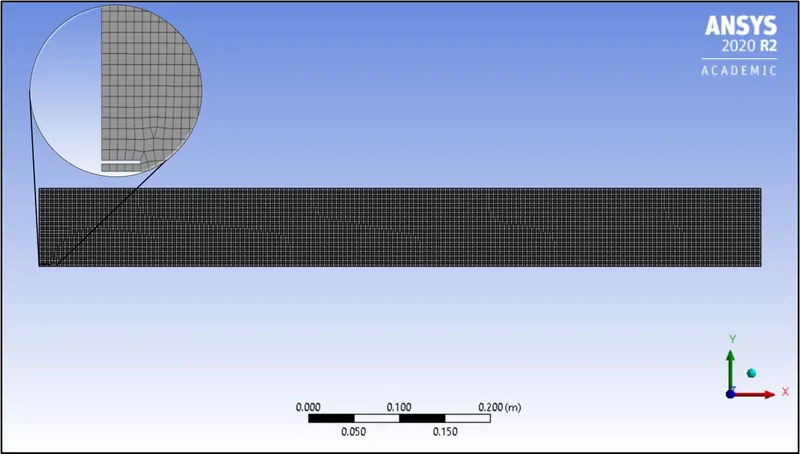
Fig. 2: Baseline Mesh
Mesh statistics and mass flow rate values at the outlet for Baseline Mesh using different Pressure-Velocity coupling schemes:
|
Mesh |
Mesh Element Size [m] |
Nodes |
Elements |
Pressure-Velocity Coupling Scheme |
Temperature - Outlet [C] |
Mass Fraction of Soot |
Mass Fraction of `NO_x` |
|
Baseline |
0.0025 |
11134 |
10777 |
SIMPLE |
1616.4875 |
1.7759378e-08 | 5.7926104e-05 |
|
Baseline |
0.0025 |
11134 |
10777 |
SIMPLEC |
322.3185 |
6.6110208e-27 | 7.5388808e-08 |
|
Baseline |
0.0025 |
11134 |
10777 |
COUPLED |
1591.3434 |
0.00028693373 | 0.00019693813 |
Table 9: Mesh statistics, temperature, and mass fraction of soot and `NO_x` values at the outlet for Baseline Mesh using different Pressure-Velocity coupling schemes
Mesh quality attributes for Baseline Mesh:
|
Mesh |
Element Quality(avg.) |
Aspect Ratio(avg.) |
Skewness(avg.) |
Orthogonal Quality(avg.) |
|
Baseline |
0.99715 |
Triangles & Quadrilaterals -1.0035 |
2.9452e-003 |
0.99991 |
Table 10: Mesh quality attributes depicting average values of element quality, aspect ratio, skewness and orthogonal quality for Baseline mesh of the combustor model
2.5.3 Mesh Refinement approach
The initial results obtained from the Baseline mesh in Section 2.5.2 Baseline Mesh with regards to the convergence behaviour of the three different algorithms, SIMPLE, SIMPLEC and COUPLED, as can be seen in Fig. 7, Fig. 8, and Fig. 9 respectively, it was observed that temperature monitor plot for COUPLED scheme demonstrated stable output well before it reached the total number of iterations of 500, however, the SIMPLE and SIMPLEC solvers required more number of iterations to indicate steady predicted values. It should be noted that the mass fraction of `NO_x` and soot monitor plots have not been displayed as their range of values are of the order of 1e-04 to 1e-07 which was being recorded close to 0 and therefore deemed difficult to observe the minute changes during the solution run. Additionally, the COUPLED solver also performed better than the two previously stated algorithms in terms of reporting the lowest value of residuals for almost all of the equations involved as opposed to the convergence limits mentioned in Table 13 (although the convergence criteria option for all equations were checked off) making the results obtained more reliable and accurate for it to be reused to solve the pressure-velocity equations for the four different meshes that were prepared to obtain a mesh independent solution. As the baseline mesh contained a structured grid of elements, the mesh refinement strategy adopted while adhering to the mesh quality attributes mentioned in Section 2.2 Meshing was to reduce the mesh element size by 20% with 'Capture Proximity' option set to 'Yes' due to the presence of the small gap including the number of cells across it to be increased by a value of 1, in every subsequent mesh iteration, to minimize errors due to numerical diffusion.
Mesh 1:
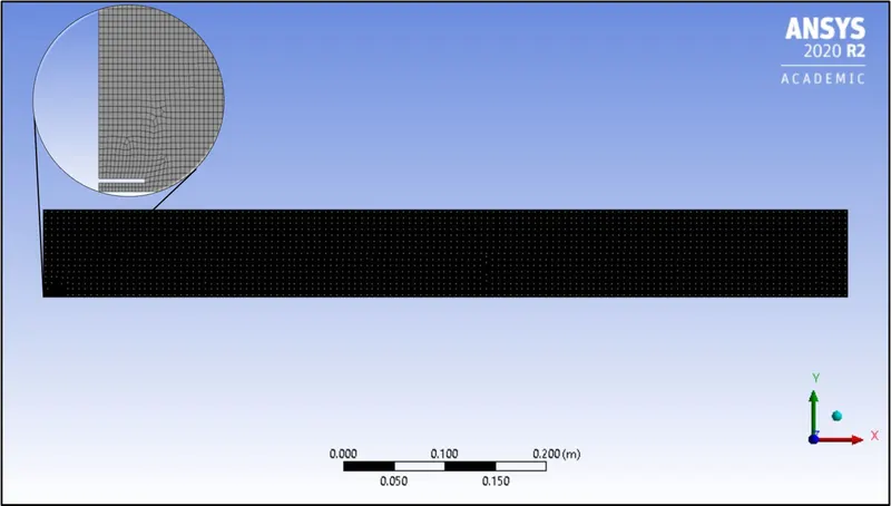
Fig. 3: Mesh 1
Mesh 2:
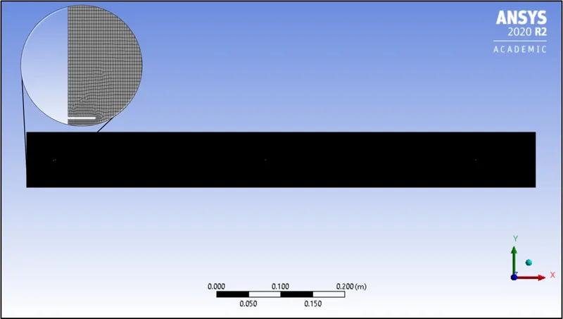
Fig. 4: Mesh 2
Mesh 3:
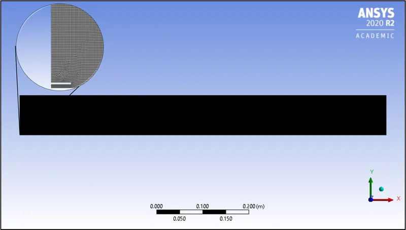
Fig. 5: Mesh 3
Mesh 4:
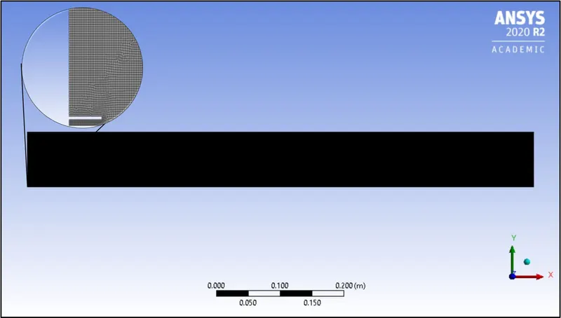
Fig. 6: Mesh 4
Mesh statistics and mass flow rate values at the outlet for different meshes using COUPLED Pressure-Velocity coupling scheme:
|
Mesh |
Mesh Element Size [m] |
Num cells across gap |
Nodes |
Elements |
Temperature - Outlet [C] |
%var |
Mass Fraction of Soot | %var | Mass Fraction of `NO_x` | %var |
|
1 |
0.0012 |
2 |
47652 |
46905 |
1588.8877 |
-- | 0.00027805464 | -- | 0.00018481136 | -- |
|
2 |
0.001 |
3 |
68325 |
67421 |
1587.7589 |
-0.0711 |
0.00031567635 | +13.5303 |
0.00018583988 |
+0.5565 |
|
3 |
0.0008 |
4 |
107158 |
106030 |
1586.9724 |
-0.0495 |
0.0003332328 | +5.5615 | 0.00018354082 | -1.2371 |
|
4 |
0.00064 |
5 |
166125 |
164714 |
1587.1194 |
-0.00926 |
0.00031938384 | -4.1559 | 0.00018399379 | +0.2468 |
Table 11: Mesh statistics, temperature, and mass fraction of soot and `NO_x` values at the outlet for different meshes using COUPLED Pressure-Velocity coupling scheme and their minimum percentage variation values with subsequent mesh
Mesh quality attributes for the four different meshes:
|
Mesh |
Element Quality(avg.) |
Aspect Ratio(avg.) |
Skewness(avg.) |
Orthogonal Quality(avg.) |
|
1 |
0.99696 |
Triangles & Quadrilaterals - 1.0022 |
3.1124e-003 |
0.99979 |
|
2 |
0.9976 |
Triangles & Quadrilaterals - 1.0037 |
2.3557e-003 |
0.9999 |
|
3 |
0.99777 |
Triangles & Quadrilaterals - 1.006 |
2.0035e-003 |
0.9999 |
|
4 |
0.99741 |
Triangles & Quadrilaterals - 1.0026 |
2.6081e-003 |
0.99988 |
Table 12: Mesh quality attributes depicting average values of element quality, aspect ratio, skewness and orthogonal quality for different meshes of the combustor model
From the meshing statistics in Table 11, mesh number 3 (or mesh 3) with 106030 elements represents a mesh independent result in terms of minimum percentage variation (%var) in the predicted values of temperature, and mass fraction of soot and `NO_x` quantities at the outlet. The %var is calculated as the ratio of the difference of the predicted values in two consecutive meshes to the predicted value of the previous mesh e.g., ((Temperature at outlet for Mesh 2 - Temperature at outlet for Mesh 1)/Temperature at outlet for Mesh 1). Results in Section 3 will only be referred with regards to the mesh independent solution i.e., Mesh 3.
2.6 Convergence Level
As mentioned earlier in Section 2.5.2 Baseline Mesh, three different schemes i.e., SIMPLE, SIMPLEC and COUPLED were compared with regards to convergence study. SIMPLE scheme is iterative in nature, robust (memory efficient) and is quicker per iteration than other pressure-based solvers. SIMPLEC scheme, similar to the SIMPLE scheme, allows increased under relaxation to the pressure correction term that improves in convergence times especially when employed in complicated flows with turbulence and/or supplementary physical models and as such offers greater diversity in terms of computational problems for implementation over SIMPLE scheme. While SIMPLE and SIMPLEC schemes are segregated type of schemes i.e., pressure and velocity terms are updated sequentially, the COUPLED scheme on the other hand updates the pressure and velocity terms simultaneously. This allows the COUPLED scheme to be more efficient in its single-phase implementation especially for steady-state flows offering superior performance over the segregated algorithms (SIMPLE and SIMPLEC) thereby requiring fewer iterations to converge. The selection of schemes for the different terms under spatial discretization includes assigning Gradient to Least Squares Cell Based scheme, pressure to second order scheme, momentum, `CH_4`, `O_2`, `CO_2`, `H_2O`, Soot, Pollutant NO, and energy to second order upwind scheme, and Turbulent Kinetic Energy and Turbulent Dissipation Rate to the first order upwind scheme. Least Squares Cell Based scheme is the default gradient method chosen by ANSYS Fluent which is used to compute the change in values across the centroid of two cells along a vector path and is a computationally less expensive scheme offering comparable accuracy to the node-based gradient scheme, both of which are superior to the cell-based gradient scheme. The second order scheme for the pressure makes use of the central differencing scheme and is generally considered to be more accurate than the Standard and Linear schemes as well as robust in the case of skewed meshes. A second order upwind scheme is chosen for the momentum, `CH_4`, `O_2`, `CO_2`, `H_2O`, Soot, Pollutant NO, and energy terms that makes use of the quantities at the cell face values to compute a cell-centered solution at the cell centroid leading to a second order accurate solution. The turbulence terms viz., Turbulent Kinetic Energy and Turbulent Dissipation Rate are set at first order upwind scheme by default which makes use of quantities at the cell faces as the cell-average value indicating that it is first-order accurate. The reason to have the turbulence terms discretized using the first-order upwind scheme as was noted in observations from simulations across different applications is because using a higher or even second order upwind scheme leads to a computationally expensive (more compute time) solution while also demonstrating stability issues in the form of repeating oscillations of values and not necessarily guaranteeing always a more accurate solution. Convergence criteria option was checked off, however, the residual values which measures the local imbalance of conserved variable in each control volume such as continuity, x-velocity, y-velocity, k, `epsilon`, `CH_4`, `O_2`, `CO_2`, `H_2O`, pollut_soot, pollut_no, and energy were monitored throughout the solution process for the defined number of iterations i.e., 500, to allow for the development of the flow behaviour which is the combustion process taking place due to turbulence driving the reaction rates determined by the eddy-dissipation model. The residual limits defined for the turbulence, species, `NO_x` and Soot model equations, and the residual and monitor plots corresponding to the different meshes are shown in the table and figures below respectively:
|
k-`epsilon` |
Species |
`NO_x` |
Soot |
|
|
continuity |
1e-03 |
-- | -- | -- |
|
x-velocity |
1e-03 |
-- | -- | -- |
|
y-velocity |
1e-03 |
-- | -- | -- |
|
energy |
1e-06 |
-- | -- | -- |
|
k |
1e-03 |
-- | -- | -- |
|
`epsilon` |
1e-03 |
-- | -- | -- |
|
`CH_4` |
-- |
0.001 | -- | -- |
|
`O_2` |
-- | 0.001 | -- | -- |
|
`CO_2` |
-- | 0.001 | -- | -- |
|
`H_2O` |
-- | 0.001 | -- | -- |
|
pollut_no |
-- | -- | 1e-06 | -- |
|
pollut_soot |
-- | -- | -- | 1e-06 |
Table 13: Residual Values of the different equations used in the Realisable k-`epsilon` turbulence model, Species model, `NO_x` model and Soot model
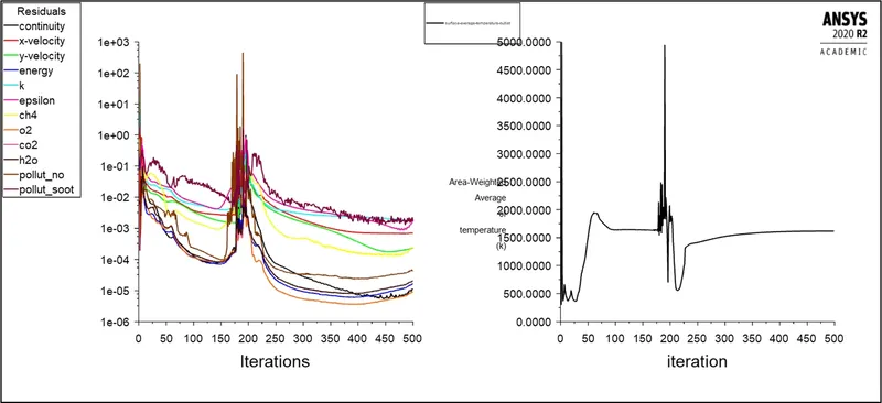 Fig. 7: Scaled Residuals and surface average temperature at the outlet plots for Baseline mesh using Realisable k-`epsilon` turbulence model and methane-air mixture model with SIMPLE solver for `CH_4` mass fraction of 1
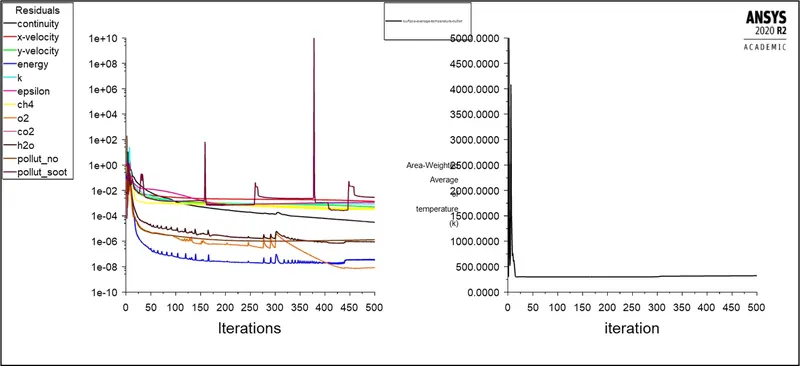
Fig. 8: Scaled Residuals and surface average temperature at the outlet plots for Baseline mesh using Realisable k-`epsilon` turbulence model and methane-air mixture model with SIMPLEC solver for `CH_4` mass fraction of 1
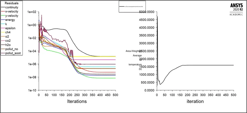
Fig. 9: Scaled Residuals and surface average temperature at the outlet plots for Baseline mesh using Realisable k-`epsilon` turbulence model and methane-air mixture model with COUPLED solver for `CH_4` mass fraction of 1
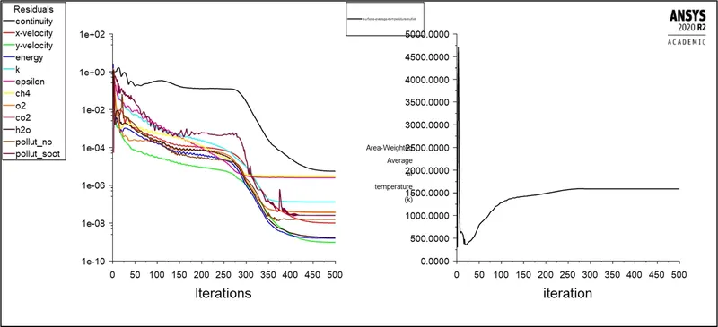
Fig. 10: Scaled Residuals and surface average temperature at the outlet plots for mesh 1 using Realisable k-`epsilon` turbulence model and methane-air mixture model with COUPLED solver for `CH_4` mass fraction of 1
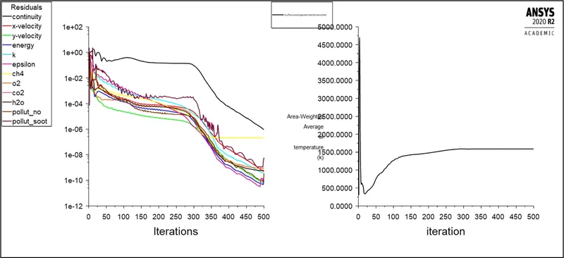
Fig. 11: Scaled Residuals and surface average temperature at the outlet plots for mesh 2 using Realisable k-`epsilon` turbulence model and methane-air mixture model with COUPLED solver for `CH_4` mass fraction of 1
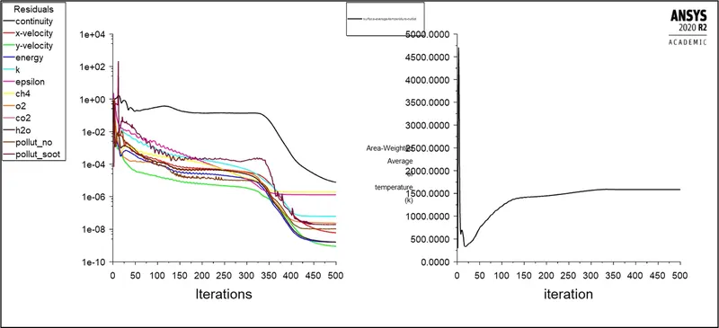
Fig. 12: Scaled Residuals and surface average temperature at the outlet plots for mesh 3 using Realisable k-`epsilon` turbulence model and methane-air mixture model with COUPLED solver for `CH_4` mass fraction of 1
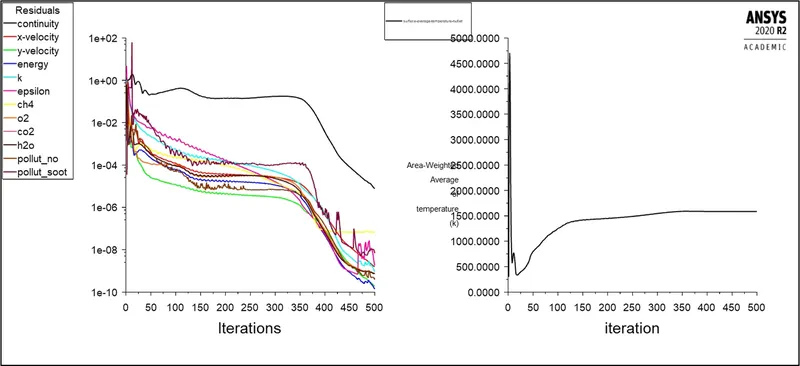
Fig. 13: Scaled Residuals and surface average temperature at the outlet plots for mesh 4 using Realisable k-`epsilon` turbulence model and methane-air mixture model with COUPLED solver for `CH_4` mass fraction of 1
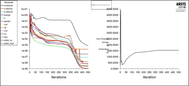
Fig. 14: Scaled Residuals and surface average temperature at the outlet plots for mesh 3 using Realisable k-`epsilon` turbulence model and methane-air-2step mixture model with COUPLED solver for `CH_4` mass fraction of 0.95 and `H_2O` mass fraction of 0.05
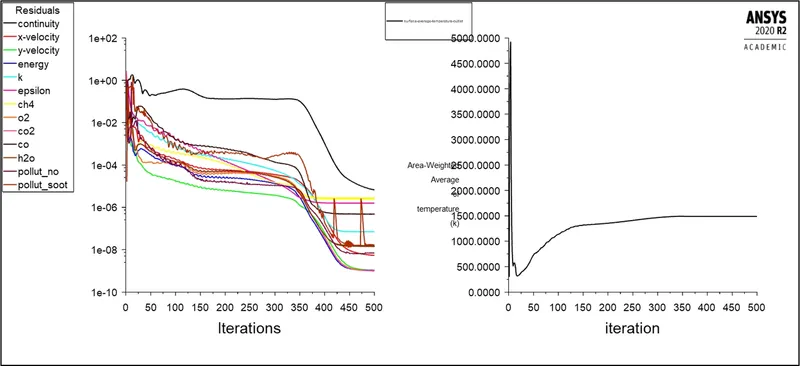
Fig. 15: Scaled Residuals and surface average temperature at the outlet plots for mesh 3 using Realisable k-`epsilon` turbulence model and methane-air-2step mixture model with COUPLED solver for `CH_4` mass fraction of 0.90 and `H_2O` mass fraction of 0.10
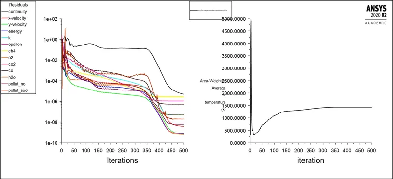
Fig. 16: Scaled Residuals and surface average temperature at the outlet plots for mesh 3 using Realisable k-`epsilon` turbulence model and methane-air-2step mixture model with COUPLED solver for `CH_4` mass fraction of 0.85 and `H_2O` mass fraction of 0.15
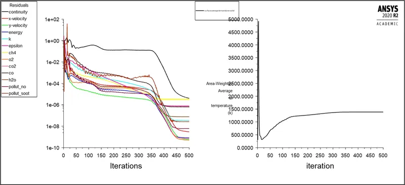
Fig. 17: Scaled Residuals and surface average temperature at the outlet plots for mesh 3 using Realisable k-`epsilon` turbulence model and methane-air-2step mixture model with COUPLED solver for `CH_4` mass fraction of 0.80 and `H_2O` mass fraction of 0.20
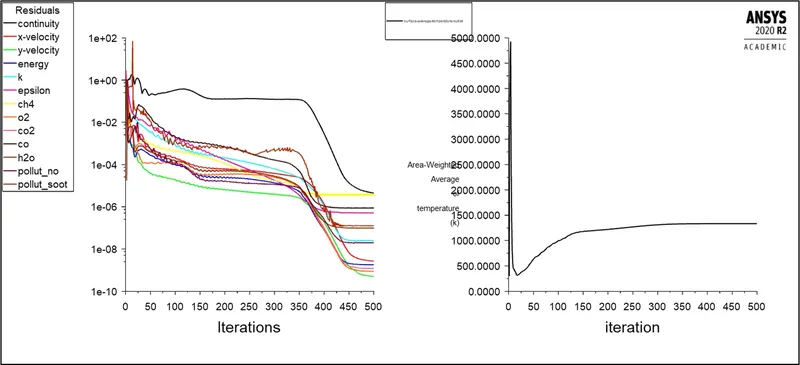
Fig. 18: Scaled Residuals and surface average temperature at the outlet plots for mesh 3 using Realisable k-`epsilon` turbulence model and methane-air-2step mixture model with COUPLED solver for `CH_4` mass fraction of 0.75 and `H_2O` mass fraction of 0.25
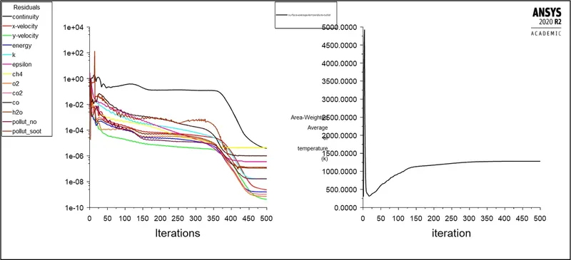
Fig. 19: Scaled Residuals and surface average temperature at the outlet plots for mesh 3 using Realisable k-`epsilon` turbulence model and methane-air-2step mixture model with COUPLED solver for `CH_4` mass fraction of 0.70 and `H_2O` mass fraction of 0.30
From Fig. 7, Fig. 8 and Fig. 9, it can be noticed that only COUPLED pressure-velocity coupling scheme had shown stable convergence with highly stable output as seen in the monitor plot well before they reach the total number of iterations indicating that a steady-state solution was obtained and had the lowest recorded residual limit values for almost all equations while taking the most computational time as was also mentioned in Section 2.5.3 Mesh Refinement approach. This reconfirms the expected behaviour from each of the schemes. A similar trend in results is also observed from Fig. 10 to Fig. 19 in the simulation of different meshes as well as different values of water content in the fuel using the COUPLED algorithm.
3. Results and Discussion
In Section 3.1, mass fraction of different species as both gradient and line plots and temperature gradient plots are highlighted along with tabulated information for temperature, and mass fraction of soot and `NO_x` values at the outlet for different values of water content in the fuel.
3.1 Effect of different values of water content in the fuel
Fig. 20 to Fig. 23 shows the mass fraction of different species and temperature as gradient plots along Plane 1 (defined in Section 2.4 Post-Processing) and Fig. 24 to Fig. 30 illustrates the mass fraction profiles of different species at different line locations as defined from Table 3 to Table 8 (Section 2.4 Post-Processing). It can be seen that with mixture model as methane-air which contains only methane mass fraction at the fuel inlet, the mass fraction of `O_2` and `CO_2` species, Pollutant NO and soot is the highest while with mixture model as methane-air-2step and for increase in the mass fraction of `H_2O` species from 5% to 30% by mole in intervals of 5 at the same boundary, the mass fraction of `O_2` and `CO_2` species, Pollutant NO and soot decreases along with lowering in temperature values. Additionally, the line plots and especially for the Pollutant NO and soot indicate the location and amount in terms of concentration from the inlet (or closer to the outlet) at which they are present within the combustor. In regards to thermal `NO_x` formation also known as the extended Zeldovich [2][4] mechanism, high temperature causes reactions between nitrogen in air with oxygen, one of them being in their molecular form and the other as an atom, as well as between atomic nitrogen and OH (hydroxyl) radicals in the case of rich fuel conditions and at near stoichiometric equilibrium. The concentration of thermal `NO_x` increases exponentially with increase in temperature and with greater concentration of `O_2` species. Prompt `NO_x` formation, initially identified by Fenimore [3][4], takes place during combustion of the hydrocarbon fuels leading to rapid reaction between hydrocarbon radicals and molecular nitrogen to produce HCN (hydrogen cyanide) and atomic nitrogen of which the atomic nitrogen combines with OH groups or radicals to create atomic hydrogen and NO. The condition favourable for Prompt `NO_x` formation is a rich fuel environment or presence of excess fuel. Soot, on the other hand, is formed as a result of the incomplete combustion of hydrocarbon fuels and particularly due to low concentration of OH radicals required for its oxidation as `O_2` gets consumed for combustion. Addition of water and especially to the fuel reduces the combustion temperature aiding in lowering the thermal `NO_x` species concentration, makes the fuel less rich which prevents the presence of residual hydrocarbon radicals thereby also lowering the prompt `NO_x` species concentration, and improves the concentration of OH radicals which gets used for the oxidation of soot implying that a more complete combustion is being attempted to achieve.
For Mesh 3:
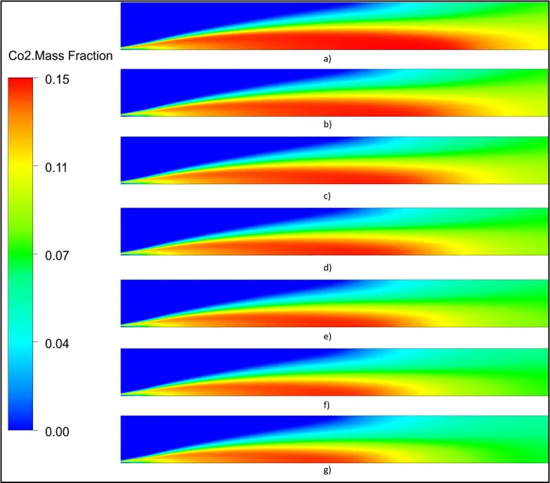
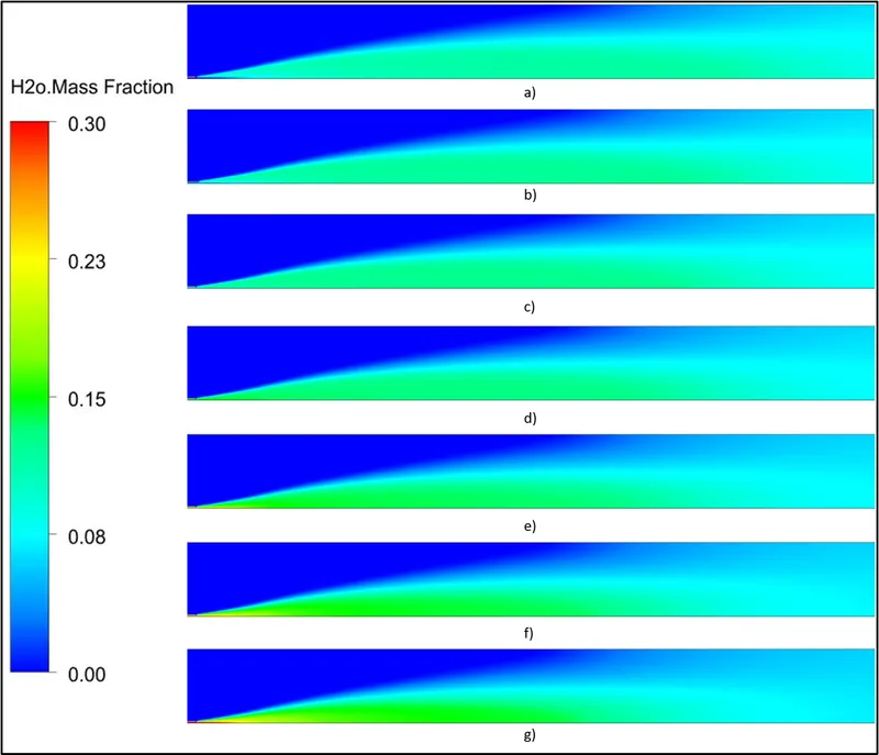 Fig. 20: `CO_2` and `H_2O` mass fraction plots along plane 1 for different water content values in the fuel by mole [a) 0%, b) 5%, c) 10%, d) 15%, e) 20%, f) 25%, g) 30%]
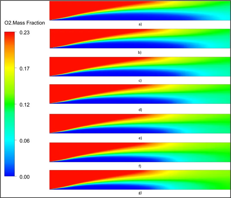
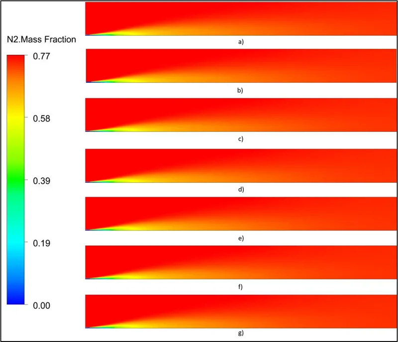 Fig. 21: `O_2` and `N_2` mass fraction plots along plane 1 for different water content values in the fuel by mole [a) 0%, b) 5%, c) 10%, d) 15%, e) 20%, f) 25%, g) 30%]
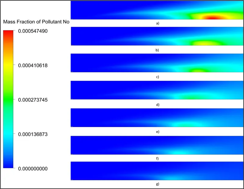
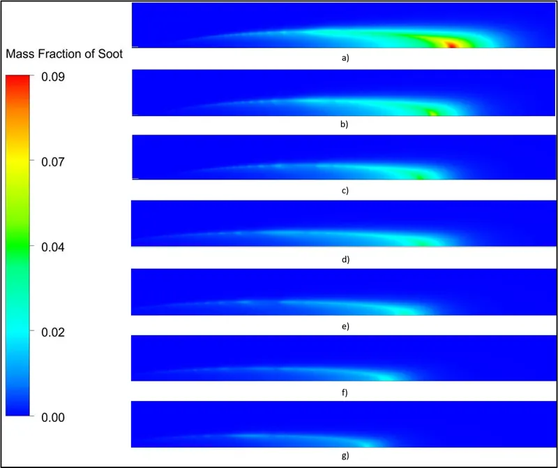 Fig. 22: `NO_x` (or Pollutant `NO`) and Soot mass fraction plots along plane 1 for different water content values in the fuel by mole [a) 0%, b) 5%, c) 10%, d) 15%, e) 20%, f) 25%, g) 30%]
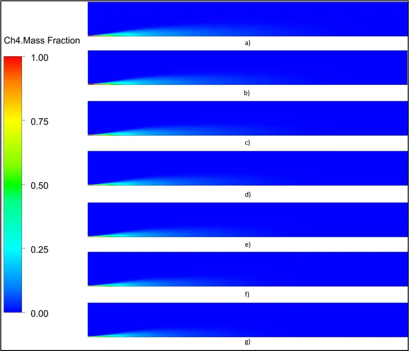
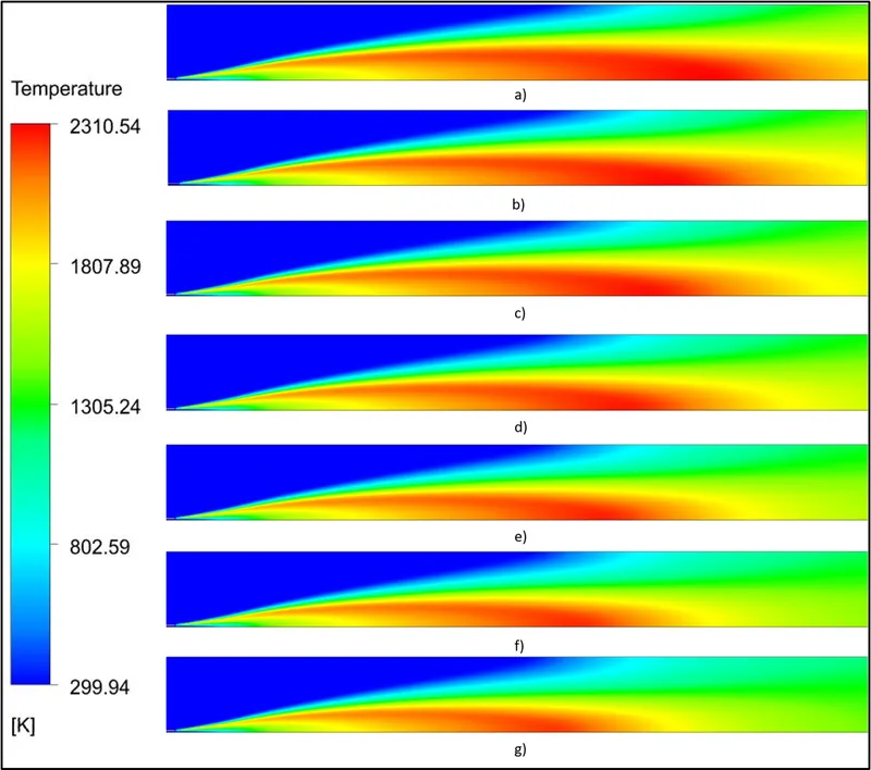 Fig. 23: `CH_4` mass fraction and temperature plots along plane 1 for different water content values in the fuel by mole [a) 0%, b) 5%, c) 10%, d) 15%, e) 20%, f) 25%, g) 30%]
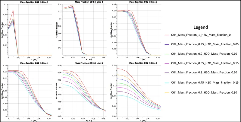
Fig. 24: `CO_2` mass fraction line plots at different line locations and water content values in the fuel by mole [a) 0%, b) 5%, c) 10%, d) 15%, e) 20%, f) 25%, g) 30%]
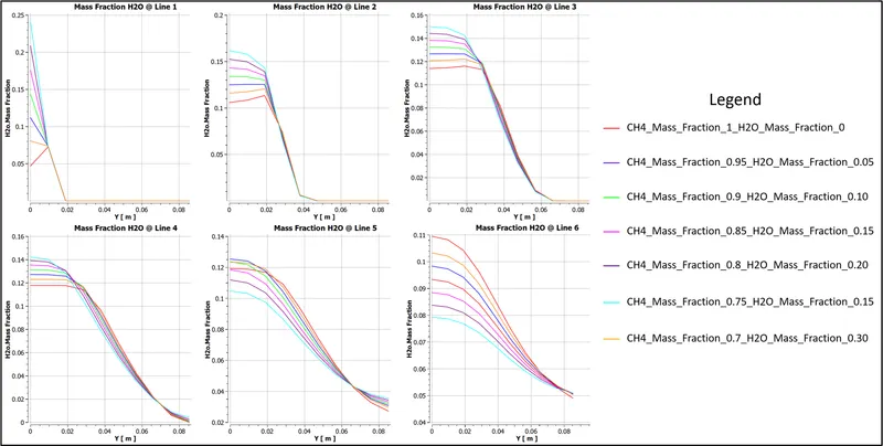
Fig. 25: `H_2O` mass fraction line plots at different line locations and water content values in the fuel by mole [a) 0%, b) 5%, c) 10%, d) 15%, e) 20%, f) 25%, g) 30%]
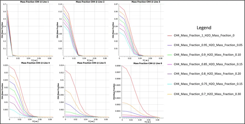
Fig. 26: `CH_4` mass fraction line plots at different line locations and water content values in the fuel by mole [a) 0%, b) 5%, c) 10%, d) 15%, e) 20%, f) 25%, g) 30%]
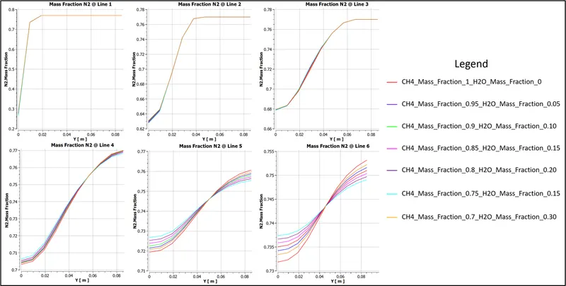
Fig. 27: `N_2` mass fraction line plots at different line locations and water content values in the fuel by mole [a) 0%, b) 5%, c) 10%, d) 15%, e) 20%, f) 25%, g) 30%]
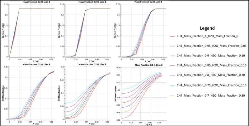
Fig. 28: `O_2` mass fraction line plots at different line locations and water content values in the fuel by mole [a) 0%, b) 5%, c) 10%, d) 15%, e) 20%, f) 25%, g) 30%]
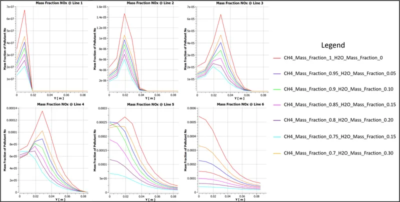
Fig. 29: `NO_x` mass fraction line plots at different line locations and water content values in the fuel by mole [a) 0%, b) 5%, c) 10%, d) 15%, e) 20%, f) 25%, g) 30%]
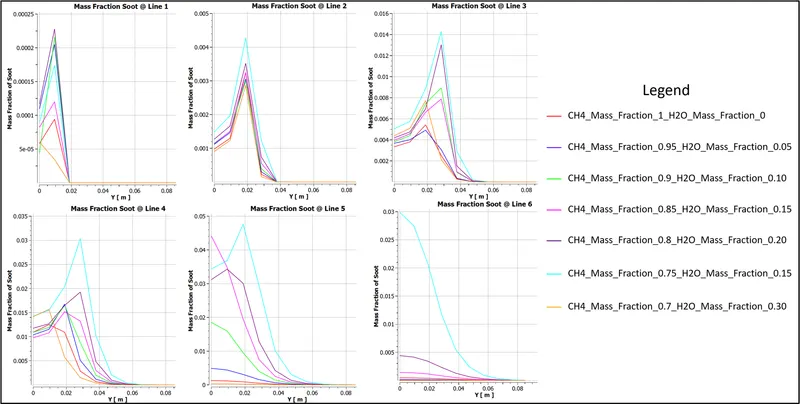
Fig. 30: Soot mass fraction line plots at different line locations and water content values in the fuel by mole [a) 0%, b) 5%, c) 10%, d) 15%, e) 20%, f) 25%, g) 30%]
|
Water content in fuel (%) |
Mass Fraction of `CH_4` |
Mass Fraction of `H_2O` |
Temperature at outlet [C] |
Mass Fraction of Soot |
Mass Fraction of `NO_x` |
|
0 |
1 |
0 |
1586.9724 |
0.0003332328 |
0.00018354082 |
|
5 |
0.95 |
0.05 |
1539.911 |
5.57e-05 |
0.00012368443 |
|
10 |
0.90 |
0.10 |
1490.3982 |
1.9e-05 |
9.59e-05 |
|
15 |
0.85 |
0.15 |
1439.6436 |
6.25e-06 |
7.24e-05 |
|
20 |
0.8 |
0.20 |
1387.5881 |
1.77e-06 |
5.30e-05 |
|
25 |
0.75 |
0.25 |
1334.1719 |
4.85e-07 |
3.75e-05 |
|
30 |
0.7 |
0.30 |
1279.2889 |
1.21e-07 |
2.55e-05 |
Table 14: Temperature, and mass fraction of soot and `NO_x` values at the outlet for different values of water content in the fuel
4. Conclusion
The numerical analysis for the given combustor model under steady state conditions for rich fuel condition and different values of water content in the fuel by mole, using the Realisable k-`epsilon` turbulence model, Species model, and `NO_x` and soot models in ANSYS Fluent 2020 R2 was well understood. It was realised that for a sufficient value of the large-eddy mixing time scale, `k/epsilon`, a combustion process could be initiated and driven by turbulence using the eddy-dissipation model, and the presence and concentration of different species, in terms of their mass fractions, involved could be visualised both along and across the combustor model. A significant decrease in mass fraction of soot and `NO_x` species was observed due to the addition of varying water content in the fuel by mole, however, this technique also tends to enhance the presence of CO (carbon monoxide) and HC levels during emissions beyond a certain limit which is its major drawback. Moreover, the water needs to be treated before being used in fuel depending on the application, which presents its own challenges in terms of storage, pumping and handling of water also varying in capacity and therefore this approach has largely been employed in standalone industrial plants that are often located near the vicinity of a large reservoir.
5. References
[1] I. M. Khan and G. Greeves. "A Method for Calculating the Formation and Combustion of Soot in Diesel Engines". In N. H.Afgan and J. M.Beer, editorsHeat Transfer in Flames. Chapter 25Scripta, Washington DC. 1974.
[2] Zeldovich, J. (1946) The oxidation of nitrogen in combustion and explosions. Acta Physicochimica URSS, 21, 577-628.
[3] C. P. Fenimore and G. W. Jones. "Oxidation of soot by hydroxyl radicals". J. Phys. Chem. 71. 593–597. 1967.
[4] ANSYS Fluent Theory Guide, Release 2020 R2 - © ANSYS, Inc. All rights reserved.