Week 5.1 - Mid term project - Solving the steady and unsteady 2D heat conduction problem
1. Introduction
The significance of heat conduction as is experienced across many engineering problems is often multi-dimensional either in the form of homogeneous or non-homogeneous heat transfer that can significantly alter thermal properties. Common examples include sudden or drastic temperature difference between the inner and outer surfaces of a glass cup when hot water is poured into it leading to cracking as a result of the built-up thermal stresses. This emphasises importance on the design of different engineering applications to rely on the characteristics of heat transfer in more than one dimension such that it can be reliable and optimised to varying physical situations. Moreover, in the case of high-power devices, the heat generation is usually transient and depending on the thermal load, conduction could also be possible. The aim of this programming exercise is to solve the steady and unsteady state 2D heat conduction problem using iterative methods viz., Jacobi, Gauss seidel and successive over-relaxation (SOR), for known temperature boundary conditions at the outermost surfaces of a square domain.
2. Method
2.1 Modelling
The problem was solved by building a mathematical model in Matlab (code snippet for which is attached with this report). Since, the domain was assumed to represent a unit square as well as the number of grid points to be same in either direction (x axis and y axis relating to a two-dimensional setup), 'linspace' function was used to generate, in this case linearly spaced equidistant vectors, by passing the domain length and width values. The values for time-step size especially with regards to the explicit scheme is calculated based on the restrictive form of the stability criterion, thermal diffusivity (or `alpha`) is considered as '1.4' as opposed to the usual range of order of 1e-3 to 1e-6 for materials like metals for attaining convergence in fewer time steps and weighted average (or extrapolation factor `omega`) for the SOR iteration method as '1.1' to demonstrate acceleration in convergence rate of the gauss-seidel iteration method with formulations and descriptions of all of them explained in detail in Section 2.2 Mathematical Model Setup, of this report. Also, iterative methods viz., Jacobi, Gauss seidel and SOR have been also used to compute temperature gradients and residual error values for steady and unsteady implicit technique.
2.2 Mathematical Model Setup
Two-dimensional transient heat conduction equation can be represented as:
`(partial T)/(partial t) + alpha*((partial^2T)/(partial x^2)+(partial^2T)/(partial y^2)) = 0` ;where (Eq. 1)
'T' is temperature described as a function of space (x,y) and time (t), and
`alpha` is thermal diffusivity
For steady state conditions, the time derivative of temperature in (Eq. 1) assumes a value of 0 as it is considered that the variation of temperature in time is negligible or in other words it can be treated as a constant. Therefore, (Eq. 1) for steady state conditions can be further simplified as follows:
`((partial^2T)/(partial x^2)+(partial^2T)/(partial y^2)) = 0 or nabla^2(T) = 0` ;where (Eq. 2)
`nabla` is divergence of temperature gradient (`nabla T`)
The steady state form of two-dimensional heat conduction equation that also represents a second order linear partial differential equation, as seen in (Eq. 2), is elliptic in nature as the difference of the square of the coefficient containing the product of the partial derivatives of x and y (let's say `B^2`), and the product of the coefficient of the terms containing the second order derivatives of x and y individually times 4 (let's say `4*A*C`) is less than 0 (i.e., `B^2-4*A*C<0`) and the solution can therefore be obtained by applying the second order central differencing scheme of the second derivative such that at any internal grid point i.e., for coordinates not representing the boundaries of the domain, the value is computed by taking into consideration the information available at its immediately adjacent grid points, in other words from the left and right coordinates along the x-axis and top and bottom coordinates along y-axis, which mathematically can be expressed below as:
`((T_L - 2*T_P + T_R)/(Delta x^2)+(T_T - 2*T_P + T_B)/(Delta y^2)) = 0` ;where (Eq. 3)
`T_P` is the temperature value at the internal grid point (i,j),
`T_L` is the temperature value at the left coordinate or grid point (i-1,j),
`T_R` is the temperature value at the right coordinate or grid point (i+1,j),
`T_T` is the temperature value at the top coordinate or grid point (i,j+1), and
`T_B` is the temperature value at the bottom coordinate or grid point (i,j-1),
Simplifying (Eq. 3); we get
`((2*T_P)/(Delta x^2)+(2*T_P)/(Delta y^2)) = ((T_L + T_R)/(Delta x^2))+((T_T + T_B)/(Delta y^2))`
OR
`T_P*((2*(Delta x^2+Delta y^2))/(Delta x^2*Delta y^2)) = ((T_L + T_R)/(Delta x^2))+((T_T + T_B)/(Delta y^2))`
Similarly, the space terms in the transient form of two-dimensional heat conduction equation, can also be discretised by using the second order central differencing scheme of the second derivative, however, for the time derivative term there are two approaches that can be adopted for the time marching solution viz., explicit and implicit time integration methods.
The explicit time integration method for the transient form of two-dimensional heat conduction equation (Eq. 2) can be expressed mathematically as shown below:
`(((T_P)^(n+1))-((T_P)^(n)))/(Delta t) + alpha*(((T_L - 2*T_P + T_R)/(Delta x^2))^(n)+((T_T - 2*T_P + T_B)/(Delta y^2))^(n)) = 0`
OR
`(T_P)^(n+1) = (T_P)^(n) + alpha*Delta t*((T_L - 2*T_P + T_R)/(Delta x^2)+(T_T - 2*T_P + T_B)/(Delta y^2))^(n) = 0` (Eq. 4)
Likewise, the implicit time integration method for the transient form of two-dimensional heat conduction equation (Eq. 2) can be expressed mathematically as shown below:
`(((T_P)^(n+1))-((T_P)^(n)))/(Delta t) + alpha*(((T_L - 2*T_P + T_R)/(Delta x^2))^(n+1)+((T_T - 2*T_P + T_B)/(Delta y^2))^(n+1)) = 0`
OR
`(T_P)^(n+1) = (T_P)^(n) + alpha*Delta t*((T_L - 2*T_P + T_R)/(Delta x^2)+(T_T - 2*T_P + T_B)/(Delta y^2))^(n+1) = 0` (Eq. 5)
In both (Eq. 4) and (Eq. 5), the term 'n' indicates the current time step while 'n+1' the next time step. The difference between the two schemes as seen from (Eq. 4) and (Eq. 5) can be observed by the values for the space terms wherein the explicit scheme takes into consideration the current time step while the implicit scheme solves for the next time step. The other major point of distinction between the two of them includes the stability criterion, which for the explicit scheme in the case of two-dimensional problem is expressed below:
`(alpha*Delta t)/dx^2+(alpha*Delta t)/dy^2 <= 0.5` (applicable for all interior nodes in rectangular, in this case square, coordinates) (Eq. 6)
A violation of the above stability criteria leads to divergence from the actual solution, more of which has been demonstrated and discussed in detail with regards to variation in time step size value in part 3 of this challenge i.e., Week 5.3 - Mid term project - Stability analysis in the unsteady problem. The implicit scheme, however, is known to be unconditionally stable but use of larger time step size values tends to affect the accuracy of the solution and the same has been shown as comparison in part 3 of this challenge. In order to determine values of temperature using the implicit scheme, which also represents a system of linear equations, there are two classes of methods that can be investigated viz., Direct Method (also known as Gaussian elimination) and Iterative Methods. The Direct Method makes use of a known number of steps to resolve final solutions in an almost systematic manner, however, this works best for a rather small set of equations as with growing complexities of different physical problems, the size of the matrices grows larger which also leads to greater constraints on memory requirements of a given computing system. This is where the second method or the iterative methods becomes advantageous as it makes use of an initial guess for the solution that is iteratively updated until the error in the solution reaches below a specified tolerance limit, as deemed fit by the user, also called the convergence criterion depending on the number of variables of interest. The different types of iterative methods used in this challenge for computing solutions of system of linear equations includes the Jacobi, Gauss-seidel and SOR methods and each of them are described briefly as follows:
- Jacobi iteration method: The Jacobi iteration method is employed on a system of linear equations for which a unique solution can be obtained and the main diagonal of the coefficient matrix has no zeros such that with every subsequent iteration, the values of the main diagonal elements are replaced by newly guessed values until a state of convergence is not achieved.
- Gauss-seidel iteration method: Similar to the Jacobi iteration method, the Gauss-seidel iteration method can be employed on a system of linear equations that has a unique solution and the leading diagonal of the coefficient matrix contains non-zero terms, however, the values along the main diagonal are replaced during the same iteration such that values to be computed at a given location that depend on them can utilise the newly guessed values unlike with Jacobi where the same process happens simultaneously. Therefore, the Jacobi iteration method is known as method of simultaneous replacements and the Gauss-seidel method as method of successive replacements.
- SOR iteration method: The SOR iteration method can be considered as an extrapolation of the Gauss-seidel method such that a weighted average is utilised between the previous iteration and the newly computed value in an attempt to improve the performance of the base solver i.e., the Gauss-seidel method, by achieving a faster rate of convergence. There are, however, limitations to the value of the weighted average (also called as the extrapolation factor) beyond which possibilities of convergence become difficult.
In order to highlight the mathematical implications of the above three iteration methods, let's consider the following system of linear equations:
`A*X = B`; where (Eq. 7)
'A' represents the coefficient matrix,
'X' is the matrix of unknowns, and
'B' is the matrix of constants
Performing splitting operation on matrix 'A' such that A = M-N and substituting the same into (Eq. 7); we get
`(M-N)*X = B` (Eq. 8)
Simplifying (Eq. 8); we get
`M*X = N*X + B` (Eq. 9)
Multiplying by `M^-1` on both sides of (Eq. 9); we get
`M^-1*M*X = M^-1*N*X + M^-1*B`
By matrix multiplication laws, `M^-1*M = I` and therefore (Eq. 9) can be rewritten as:
`I*X = X = M^-1*N*X + M^-1*B` (Eq. 10)
For the same system of linear equations in (Eq. 7), the relation between new guess values and old guessed values can be mathematically expressed as shown below:
`X^(NEW) = T*X^(OLD) + B`; where (Eq. 11)
'T' refers to the iteration number
At a particular value of 'T', the newly generated guess values will be approximately equal to the old guessed values, such that a converged solution is obtained for which (Eq. 11) can be further reduced to the following form:
`X = T*X + B` or `X(I-T) = C` (Eq. 12)
(Eq. 12) above appears similar to the system of linear equations as seen in (Eq. 7) for which a solution would exist if matrix 'A', or in this case matrix 'I-T' is non-singular. On a closer comparison with (Eq. 10), it can be deduced that `M^-1*N = T` and `M^-1*B = C`. The values adopted by M and N represents either of the Jacobi iterative method, Gauss-seidel method or the SOR method such that their mathematical expressions take the following form:
Jacobi iteration method:
`T = D^-1(L+u)`, `C = D^-1*B`, and (Eq. 13)
`X_i^(k+1) = 1/(a(i,i))*[b_i - sum_(j ne i, j=1)^(n)a_(i,j)*X_j^k ]` (Eq. 14)
Gauss-seidel iteration method:
`T = (D-L)^-1*u`, `C = (D-L)^-1*B`, and (Eq. 15)
`X_i^(k+1) = 1/(a(i,i))*[b_i - sum_(j = 1)^(i-1)a_(i,j)*X_j^(k+1) - sum_(i = i+1)^(n)a_(i,j)*X_j^k]` (Eq. 16)
SOR iteration method:
`T = (D-omega*L)^-1*u*[omega*U+(1-omega)*D]`, `C = omega*(D-omega*L)^-1*B`, and (Eq. 17)
`X_i^(k+1) = omega*overline X_i^(k+1) + (1-omega) X_i^(k)` (Eq. 18)
For the above set of eqns. 13-18, the notations used represent the following terms:
D, L and U are diagonal, lower diagonal and upper diagonal matrices,
`a_(i,i)` and `a_(i,j)` are the values of the coefficient matrix 'A' corresponding to the concerned i and j values,
`omega` is the weighted average value or the extrapolation factor,
'k' and 'k+1' indicate the current and next generation for guess values, and
`overline X_i` in (Eq. 18) is the Gauss-seidel iterate
2.3 Post-Processing
In order to plot the temperature gradients across the domain space and residual error plots based on the given boundary conditions and calculated time-step size value, Matlab's in-built pseudocolor (or pcolor) and semilogy plot functions were used respectively. As the name suggests, the pseudocolor plot displays the data of the intended values, in this case temperature, as a set of coloured cells across the grid defined by the range of x and y coordinates such that the numerical data in the temperature matrix specifies its colour at the vertices and the colour assumed by a particular face is directly dependent on the colour of its neighbouring four vertices. The semilogy plot on the other hand plots x-coordinates as a linear scale along the x-axis while values on the y-axis as a base-10 logarithmic scale of its y-coordinate values which in this case relates to the error values whose order of magnitude reaches as low as 10e-13 thereby allowing for better visualisation with regards to drawing inferences on converged state solutions of temperature. For each iterative solver in the steady state technique, an animation file of type '.avi' was also captured and converted as a gif file for improved file compression to show the variation in residual error values as new values of steady state temperature are calculated and old values of the same updated which can be viewed in Section 3, Results. Similarly, an animation file of type '.avi' was also captured and converted as a gif file for the unsteady state solutions, however, due to the large file sizes and issues in compressing the obtained gif file further that retained sufficient quality and frame rates, the same was not possible to be displayed for visualisation and hence also discarded from the Matlab code. A legend, title, textbox (represented by varying iteration number or total time-step and execution time values during the space and time marching), and x and y labels have been added for a better understanding of the graphical representation.
3. Results
3.1 Computed values of temperature gradients and residual error for steady and unsteady state (explicit and implicit techniques) using different iterative solvers
The figures below (Fig.1 - Fig.7) shows the temperature gradients and residual error values computed for steady and unsteady state (explicit and implicit techniques) using different iterative solvers. The residual error values were determined by computing the maximum of the absolute difference across all the elements of the previous iteration matrix and current iteration matrix (previous time step and current time step in the case of unsteady state explicit technique) containing the temperature values. The residual error values calculated for the unsteady state explicit technique were only performed to highlight number of time steps required before the error reaches below the specified tolerance limit of 1e-4 in order to enable comparison against the steady state and unsteady state implicit technique solutions. It can be seen that the number of iterations required by the iterative solvers for both solutions of steady and unsteady state implicit technique (for the first time step) are of the order; Jacobi > Gauss seidel > SOR while the unsteady state explicit technique requires the most time steps before the residual error values crosses the tolerance limit. Additionally, in the case of the unsteady state (explicit and implicit techniques), the solvers were allowed to compute a solution until all values between previous time step and recently updated time step exactly match each other i.e., their difference is 0, upon which the time loop was terminated as opposed to continuing upto a pre-defined limit of 1400 time steps and it can be observed that the explicit technique attains the aforementioned condition at an earlier number of time steps at 574 as compared to the implicit technique based on the number of iterations for any of the iterative methods viz., Jacobi (Total number of iterations = 2876), Gauss seidel (Total number of iterations = 2109) and SOR (Total number of iterations = 2500). It should be noted that the execution time depends on the load on the computational resources of the given system at a particular instant and may vary for every new program run and a comparison between number of time steps for the unsteady state (explicit and implicit techniques) as well as number of iterations against the steady state solution has been provided in part 2 of this challenge i.e., Week 5.2 - Mid term project - Steady vs unsteady state analysis, and that differences between number of time steps and iterations were highlighted in the current challenge to differentiate between the performance of the iterative methods.
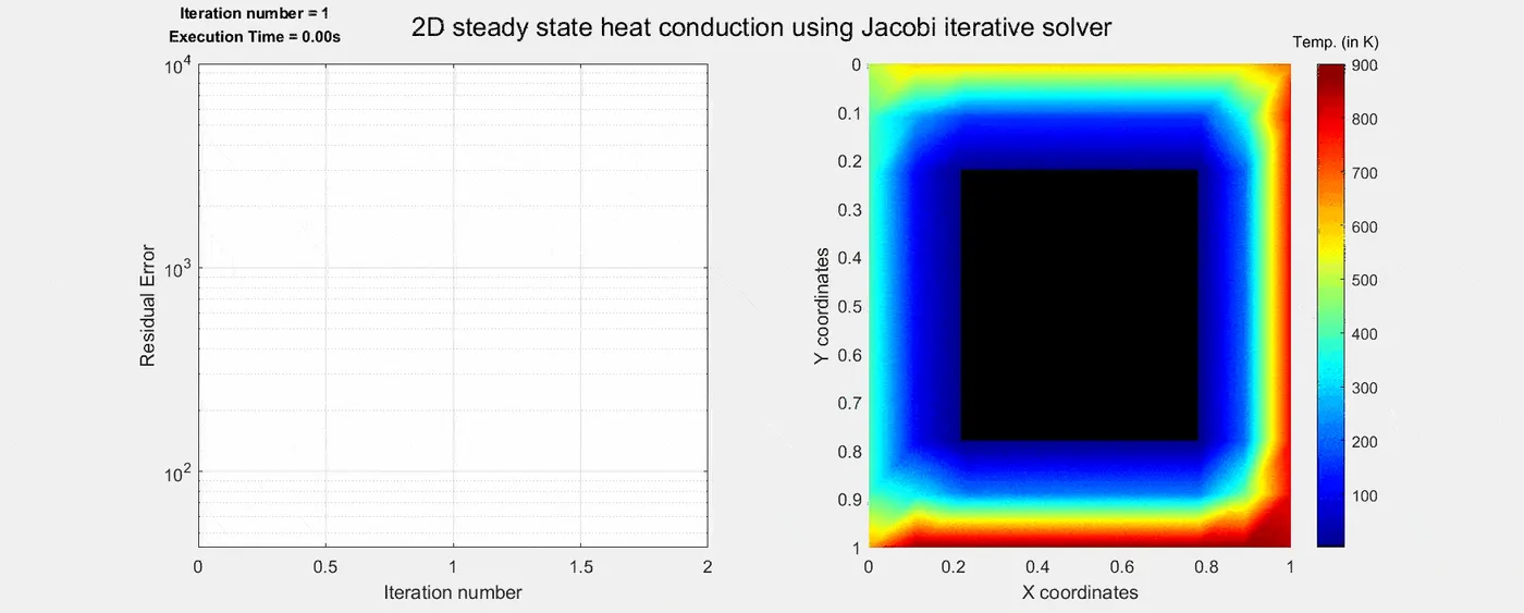
Fig. 1: 2D steady state heat conduction using Jacobi iterative solver (Iterations for convergence = 216)
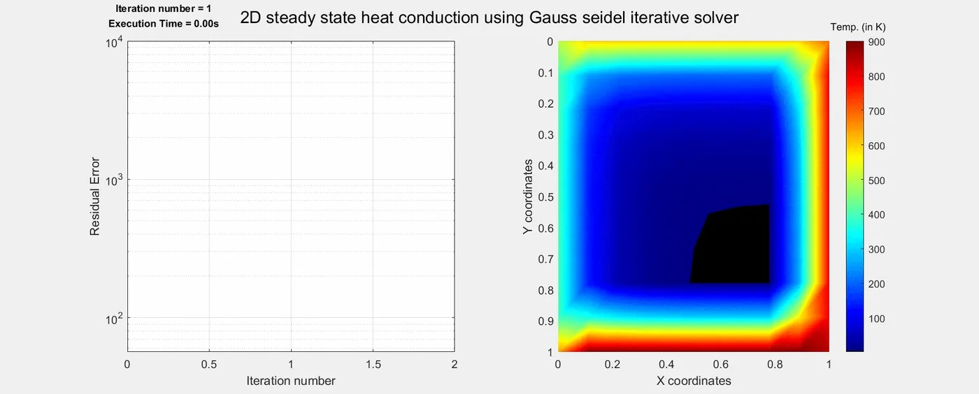
Fig. 2: 2D steady state heat conduction using Gauss seidel iterative solver (Iterations for convergence = 116)
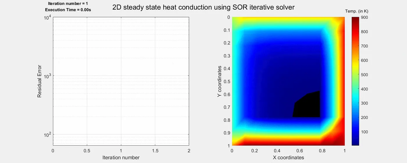
Fig. 3: 2D steady state heat conduction using SOR iterative solver (Iterations for convergence = 95)
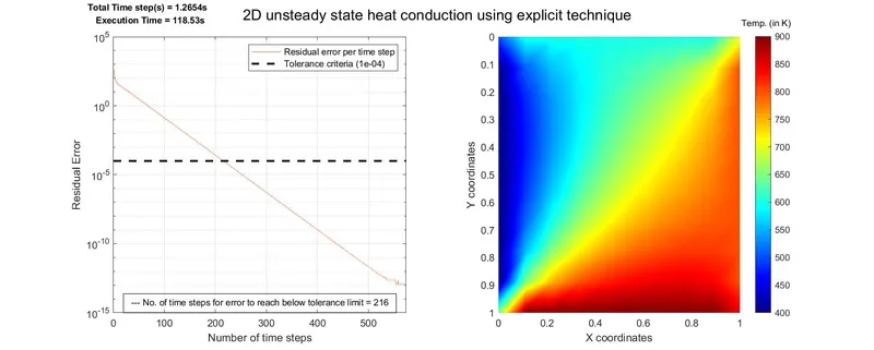
Fig. 4: 2D unsteady state heat conduction using explicit technique
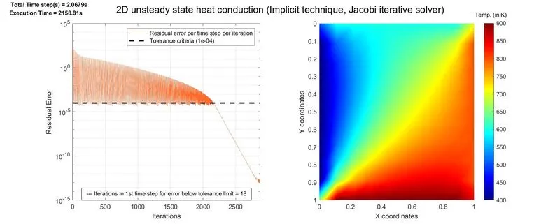
Fig. 5: 2D unsteady state heat conduction using implicit technique and Jacobi iterative solver
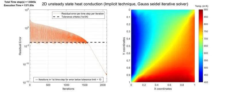
Fig. 6: 2D unsteady state heat conduction using implicit technique and Gauss seidel iterative solver
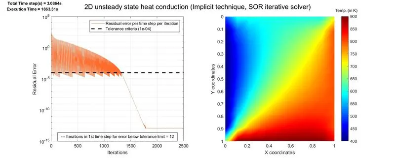
Fig. 7: 2D unsteady state heat conduction using implicit technique and SOR iterative solver
4. Discussion
The evaluation of temperature gradients for steady and unsteady state solutions using different iterative methods shows that the Jacobi method takes most number of iterations to reach a state of convergence followed by the Gauss seidel method and then the SOR method. As explained in Section 2.2 Mathematical Model Setup, variation in results with respect to attaining convergence based on number of iterations arise from the difference with regards to the manner by which the guess values are treated i.e., Gauss seidel iterative method takes into account the recently computed guessed values at positions of the matrix for which information is available in the same iteration to compute new guess values for locations that depend on it while the Jacobi iterative method continues to use the previously computed guessed values or guess values pertaining to the earlier iteration. The SOR method, based on the Gauss seidel method, uses the weighted average value (also called as extrapolation factor or in this case over-relaxation factor) and evaluates new guess values that tend to produce more appropriate guess values thereby enhancing the rate of convergence. Variation in the value of the extrapolation factor in an attempt to achieve improved convergence rate has been highlighted and discussed in part 2 of this challenge i.e., Week 5.2 - Mid term project - Steady vs unsteady state analysis. Since, the unsteady state explicit scheme requires the time step size to be determined such that its value does not violate the stability criterion, the evaluation of the same was based on its restrictive form, which implies that depending on the desired level of accuracy for the solution, a certain degree of relaxation in the value of the time step size may be allowed for the implicit technique as it is unconditionally stable for a faster rate of convergence while also ensuring the solution does not tend to instability.
5. Conclusion
Solution for steady and unsteady state 2D heat conduction problem using iterative methods in Matlab was well understood with this programming exercise. It was realised that based on appropriate values of extrapolation factor, the iterative methods generally followed a trend wherein the Jacobi method required most number of iterations followed by the Gauss seidel method and then the SOR method before achieving convergence. Moreover, the value of time-step size with regards to the stability criterion especially for the unsteady state explicit technique and because the temperature values eventually attain a steady state solution, the time-marching using the transient process is computationally expensive than a steady state approach.
CODE:
Program to solve two-dimensional steady and unsteady heat conduction problem that uses first order forward differencing for the time derivative and second order central differencing for the space term.
close all
clear all
clc

%% Inputs for the steady and unsteady 2D heat conduction problem

% Domain Length and Width (Given that the domain is a unit square)
[L,W] = deal(1);

% Number of grid points along x and y directions
[n_x,n_y] = deal(10);

% Initialising temperature arrays for steady and unsteady state analysis
[T_steady, T_explicit, T_implicit, T] = deal(ones(n_x,n_y));

% Boundary Conditions
% Temperature
[T_steady(1:end,1),T_explicit(1:end,1),T_implicit(1:end,1),T(1:end,1)] = deal(400);
[T_steady(1,1:end),T_explicit(1,1:end),T_implicit(1,1:end),T(1,1:end)] = deal(600);
[T_steady(1:end,end),T_explicit(1:end,end),T_implicit(1:end,end),T(1:end,end)] = deal(800);
[T_steady(end,1:end),T_explicit(end,1:end),T_implicit(end,1:end),T(end,1:end)] = deal(900);
[T_steady(1,end),T_explicit(1,end),T_implicit(1,end),T(1,end)] = deal((T(1,end-1)+T(2,end))/2);
[T_steady(end,end),T_explicit(end,end),T_implicit(end,end),T(end,end)] = deal((T(end,end-1)+T(end-1,end))/2);
[T_steady(end,1),T_explicit(end,1),T_implicit(end,1),T(end,1)] = deal((T(end-1,1)+T(end,2))/2);
[T_steady(1,1),T_explicit(1,1),T_implicit(1,1),T(1,1)] = deal((T(1,2)+T(2,1))/2);

% Creating a backup of temperature values

[Told_steady,Told_explicit,Told_implicit, T_prev_dt]  = deal(T);

% Creating mesh using linspace command

x = linspace(0,L,n_x);
y = linspace(0,W,n_y);

% Defining the smallest length and width element of the domain
dx = abs(x(2)-x(1));
dy = abs(y(2)-y(1));

% Creating a character array of the different solver types and allocating
% one of them as the option selected for the analysis

Iterative_solver_type = {'Jacobi','Gauss seidel','SOR'};

selected_iterative_solver = string(Iterative_solver_type(1));

% Defining initial error, tolerance, iteration number and execution time,
% and thermal_diffusivity and alpha_SOR values as well as initial values of
% terms that would be used in different techniques and solvers to report
% final outcomes of variables of interest

k = 2*(dx^2+dy^2)/(dx^2*dy^2);
error = 9e9;
tol = 1e-4;
alpha_SOR = 1.1;
thermal_diffusivity = 1.4;
d = 0;
iteration_number = 1;
total_iterations = 1;
execution_time = 0;
minimum_time_steps_error_below_tol = 0;
minimum_iterations_error_below_tol = 0;

% Determination of time-step size 'dt'
% Based on the stability criteria for all interior nodes of a rectangular,
% in this case, square domain:
% (thermal_diffusivity*dt)/dx^2+(thermal_diffusivity*dt)/dy^2 <= 0.5
% Assuming the most restrictive form to ensure that all temperature
% coefficients of the current and next time step are greater than or equal
% to 0, we consider: (thermal_diffusivity*dt)/dx^2+(thermal_diffusivity*dt)/dy^2 = 0.5
dt = (0.5*dx^2*dy^2)/(thermal_diffusivity*(dx^2+dy^2));

% Simplification of terms for solution of the transient equation
k1 = (thermal_diffusivity*dt)/dx^2;
k2 = (thermal_diffusivity*dt)/dy^2;
term1 = (1+(2*k1)+(2*k2))^-1;
term2 = k1*term1;
term3 = k2*term1;

tic

%% Steady State Solution
% Week_5_Steady_2D_heat_conduction_method function to solve 2nd order
% 2 dimensional PDE (Steady State Equation):
% (d^2(T)/d(x)^2)+(d^2(T)/d(y)^2) = 0

[iteration_number_steady_state_array,error_update_steady_state_array_value,T_steady,execution_time_steady_state] = Week_5_steady_2D_heat_conduction_method(x, y, n_x, n_y, T_steady, Told_steady,dx,dy,selected_iterative_solver,k,error,tol,alpha_SOR,iteration_number,execution_time);

%% Transient State Solution
% Week_5_Steady_2D_heat_conduction_method function to solve 2nd order
% 2 dimensional PDE (Transient State Equation):
% d(T)/d(t) + alpha*(d^2(T)/d(x)^2)+(d^2(T)/d(y)^2) = 0

% Explicit Form

[time_step_number_unsteady_state_explicit_array,error_update_unsteady_state_explicit_array_value,T_explicit,execution_time_explicit_state] = Week_5_unsteady_explicit_2D_heat_conduction_method(x, y, n_x, n_y, T_explicit, Told_explicit,dx,dy,dt,error,tol,minimum_time_steps_error_below_tol,thermal_diffusivity,execution_time);

% Implicit Form

[total_iterations_time_step_unsteady_state_implicit,error_unsteady_state_implicit] = deal(ones(1));

[total_iterations_time_step_unsteady_state_implicit,time_steps,error_unsteady_state_implicit,T_implicit,execution_time_implicit_state] = Week_5_unsteady_implicit_2D_heat_conduction_method(x, y, n_x, n_y, selected_iterative_solver, T_implicit, Told_implicit, T_prev_dt, d, total_iterations_time_step_unsteady_state_implicit, error_unsteady_state_implicit, dt, error, tol, minimum_iterations_error_below_tol,alpha_SOR, term1, term2, term3, iteration_number, total_iterations, execution_time);

total_execution_time = toc;

tic

%% Combined Plots

% Creating a figure and defining its size based on positional limits

figure_combined=figure('Position', [46,115,1168,469]);

% Creating textbox for values of total code execution time inside the
% figure and iteration time/number of time steps inside the residual error
% plot at pre-determined positional limits

str_total_execution_time = strcat('Total Execution Time = ',{' '},num2str(round(total_execution_time,2)),'s');

text_box_total_execution_time = annotation('textbox', [0.82 0.951 0.165 0.054], ...
            'String', str_total_execution_time, ...
            'EdgeColor', 'none', ...
            'HorizontalAlignment', 'center','VerticalAlignment', 'top', ...
            'FitBoxToText','on');
            text_box_total_execution_time.FontSize = 9;
            text_box_total_execution_time.FontWeight = 'bold';

% Creating subplot within the main figure using psuedocolour or pcolor to
% display temperature data based on jet colour scheme for steady state
% technique as the final converged solution for all techniques and/or
% solvers based on stable solution output will appear as that represented
% by the steady state values

subplot(1,2,2);
pcolor(x,y,T_steady);
shading interp;
set(gca, 'clim', [min(T_steady, [], 'all') max(T_steady, [], 'all')]);
set(gca, 'Ydir', 'reverse')
xlabel('X coordinates');
ylabel('Y coordinates');
colormap([0 0 0; jet]);
cb = colorbar;
cb.Title.String='Temp. (in K)';
cb.Title.Position(1,1:2) = [10.85,285.65];

% Creating subplot within the main figure using semilogy to display
% residual error as a function of iterations/number of time steps for all
% the three techniques i.e., steady, unsteady explicit and unsteady
% implicit, with regards to the selected solver

subplot(1,2,1);
semilogy(iteration_number_steady_state_array,error_update_steady_state_array_value,'-r','LineWidth', 2)
grid on
hold on
semilogy(time_step_number_unsteady_state_explicit_array,error_update_unsteady_state_explicit_array_value,'-b','LineWidth', 2)
semilogy(total_iterations_time_step_unsteady_state_implicit,error_unsteady_state_implicit,'-g')
semilogy([0,max(max(length(iteration_number_steady_state_array),length(time_step_number_unsteady_state_explicit_array)),length(total_iterations_time_step_unsteady_state_implicit))],[tol,tol],'k--', 'LineWidth', 2);

if selected_iterative_solver == "SOR"
    iteration_time_step_stats = [subplot(1,2,1).Position(1)*1.65 subplot(1,2,1).Position(2)*3.6 subplot(1,2,1).Position(3)*0.75 subplot(1,2,1).Position(4)/6.6];
else
    iteration_time_step_stats = [subplot(1,2,1).Position(1)*1.7 subplot(1,2,1).Position(2)*1.25 subplot(1,2,1).Position(3)*0.75 subplot(1,2,1).Position(4)/6.6];
end

text_box_iteration_time_steps_statistics = annotation('textbox',...
    iteration_time_step_stats,...
    'VerticalAlignment','bottom',...
    'String',{['{\color{red}',char(8212),'} Iterations = ',num2str(iteration_number_steady_state_array(end))],...
    ['{\color{blue}',char(8212),'} Total Time steps = ',num2str(time_step_number_unsteady_state_explicit_array(end))],...
    ['{\color{green}',char(8212),'} Total Iterations = ',num2str(length(total_iterations_time_step_unsteady_state_implicit)),', Total Time steps = ',num2str(time_steps)]},...
    'HorizontalAlignment','left','FitBoxToText','on',...
    'FontSize',9,...
    'EdgeColor','black');

xlim([0 max(max(iteration_number_steady_state_array(end),time_step_number_unsteady_state_explicit_array(end)),max(total_iterations_time_step_unsteady_state_implicit))])
xlabel('Iteration number, No. of time steps (unsteady state, explicit)');
ylabel('Residual Error');
legend_text_1 = sprintf('Steady state, %s solver',selected_iterative_solver);
legend_text_2 = sprintf('Unsteady state, explicit technique');
legend_text_3 = sprintf('Unsteady state, implicit technique, %s solver',selected_iterative_solver);
legend_text_4 = sprintf('Tolerance criteria (%.e)',tol);
legend(legend_text_1,legend_text_2,legend_text_3,legend_text_4);
title_text = sprintf("Steady and unsteady 2D heat conduction problem");
sgtitle(title_text)

% Save converged steady-state temperature gradient and residual error plots
% of steady and unsteady state techniques (implicit and explicit)
saveas(figure_combined,sprintf('Week_5_steady_unsteady_2D_heat_conduction_final_state_solutions_using_%s_iterative_solver.jpg',selected_iterative_solver));
% close(figure_combined);
Week_5_steady_2D_heat_conduction_method to calculate steady state temperature values based on the selected solver
% Week_5_steady_2D_heat_conduction_method to calculate steady state
% temperature values based on the selected solver

function [iteration_number_steady_state_array,error_update_steady_state_array_value,T_steady,execution_time] = Week_5_steady_2D_heat_conduction_method(x, y, n_x, n_y, T_steady, Told_steady,dx,dy,selected_iterative_solver,k,error,tol,alpha_SOR,iteration_number,execution_time)

% Creating array to store error values that would be accessed in the main
% program 'Week_5_Mid_term_project_steady_unsteady_2D_heat_conduction.m' to
% plot against error values of other techniques but same solver

error_update_steady_state_array_value(1,iteration_number) = error;

% Creating a figure and defining its size based on positional limits

figure_steady_state=figure('Position', [46,115,1168,469]);

% Creating textbox with initial values of iteration numbers and code
% execution time inside the figure at pre-determined positional limits
% as well as title of the plot

str_iteration_number = strcat('Iteration number = ',{' '},num2str(iteration_number));

str_execution_time = strcat('Execution Time = ',{' '},num2str(execution_time),'s');

text_box_iteration_number = annotation('textbox', [0.102 0.951 0.13 0.054], ...
            'String', str_iteration_number, ...
            'EdgeColor', 'none', ...
            'HorizontalAlignment', 'center', ...
            'FitBoxToText','on');
            text_box_iteration_number.FontSize = 9;
            text_box_iteration_number.FontWeight = 'bold';

text_box_execution_time = annotation('textbox', [0.102 0.914 0.13 0.054], ...
            'String', str_execution_time, ...
            'EdgeColor', 'none', ...
            'HorizontalAlignment', 'center', ...
            'FitBoxToText','on');
            text_box_execution_time.FontSize = 9;
            text_box_execution_time.FontWeight = 'bold';

title_text = sprintf("2D steady state heat conduction using "+selected_iterative_solver+" iterative solver");

% Creating an animation file of format type .avi

animation_file_name = strcat(convertStringsToChars(title_text),'.avi');

obj = VideoWriter(animation_file_name);
obj.Quality = 100;
obj.FrameRate = 20;
obj.open();

tic

% Iterative solver loop

    while error>tol

        % Function call to T_steady_update to return temperature values
        % based on selected solver type

        T_steady = T_steady_update(selected_iterative_solver,n_x,n_y,dx,dy,T_steady,Told_steady,k,alpha_SOR);

        % Calculating error value as maximum of absolute difference between
        % old steady state values and updated steady state values

        error = max(abs(Told_steady-T_steady), [], 'all');

        % Updating the error array with recently calculated error values

        error_update_steady_state_array_value(1,iteration_number) = error;

        % Updating the old steady state values with updated steady state
        % values to aid in convergence

        Told_steady = T_steady;

        % Creating subplot within the main figure using psuedocolour or
        % pcolor to display temperature data based on jet colour scheme

        subplot(1,2,2);
        pcolor(x,y,T_steady);
        shading interp;
        set(gca, 'clim', [min(T_steady, [], 'all') max(T_steady, [], 'all')]);
        set(gca, 'Ydir', 'reverse')
        xlabel('X coordinates');
        ylabel('Y coordinates');
        colormap([0 0 0; jet]);
        c = colorbar;
        c.Title.String='Temp. (in K)';
        c.Title.Position(1,1:2) = [10.85,285.65];

        % Updating iteration number and storing the same to be accessed
        % later in the main program:
        % 'Week_5_Mid_term_project_steady_unsteady_2D_heat_conduction.m' to
        % plot against iterations/time steps of other techniques but same
        % solver

        iteration_number = iteration_number + 1;
        iteration_number_steady_state_array = 1:iteration_number-1;

        % Creating subplot within the main figure using semilogy to display
        % residual error as a function of iterations

        subplot(1,2,1);
        semilogy(iteration_number_steady_state_array,error_update_steady_state_array_value,'Color',[1 0.411764705882353 0.16078431372549])
        grid on
        hold on
        xlim([0 iteration_number])
        xlabel('Iteration number');
        ylabel('Residual Error');
        sgtitle(title_text)
        text_box_iteration_number.String = sprintf("Iteration number = %d",iteration_number-1);
        text_box_execution_time.String = sprintf("Execution Time = %.2fs",execution_time);
        pause(0.03)

        % Updating execution time with the elapsed time value
        execution_time = toc;

        % Capturing the recent frame and passing the same into the
        % writeVideo function to append it to obj

        f = getframe(gcf);
        writeVideo(obj,f);
    end

toc

obj.close();

% Converting the .avi format file to .gif file for improved file
% compression value

vrinfo = VideoReader(animation_file_name);
gif_file_name = strcat(convertStringsToChars(title_text),'.gif');
mov1 = VideoReader(animation_file_name);
vidFrames = read(mov1);
for n = 1:vrinfo.NumFrames
      [imind,cm] = rgb2ind(vidFrames(:,:,:,n),255);
      if n == 1
          imwrite(imind,cm,gif_file_name,'gif', 'Loopcount',inf);
      else
          imwrite(imind,cm,gif_file_name,'gif','WriteMode','append');
      end
end

% Save converged temperature gradient and residual error plots
saveas(figure_steady_state,sprintf('Week_5_steady_state_%s_solver_iteration_number_%d.jpg',selected_iterative_solver,(iteration_number-1)));
close(figure_steady_state);

% Function to calculate and update T values based on the selected solver

    function selected_solver_steady = T_steady_update(selected_iterative_solver,n_x,n_y,dx,dy,T_steady,Told_steady,k,alpha_SOR)
        if selected_iterative_solver == "Jacobi"
           for i = 2:n_x-1
               for j = 2:n_y-1
                    T_steady(i,j) = (1/k)*(((Told_steady(i-1,j)+Told_steady(i+1,j))/dx^2)+((Told_steady(i,j-1)+Told_steady(i,j+1))/dy^2));
               end
           end
        elseif selected_iterative_solver == "Gauss seidel"
                for i = 2:n_x-1
                    for j = 2:n_y-1
                        T_steady(i,j) = (1/k)*(((T_steady(i-1,j)+T_steady(i+1,j))/dx^2)+((T_steady(i,j-1)+T_steady(i,j+1))/dy^2));
                    end
                end
        else
                for i = 2:n_x-1
                    for j = 2:n_y-1
                        T_steady(i,j) = (1-alpha_SOR)*Told_steady(i,j) + alpha_SOR*((1/k)*(((T_steady(i-1,j)+T_steady(i+1,j))/dx^2)+((T_steady(i,j-1)+T_steady(i,j+1))/dy^2)));
                    end
                end
        end
        selected_solver_steady = T_steady;
    end

end
Week_5_unsteady_explicit_2D_heat_conduction_method to calculate unsteady state temperature values based on the explicit technique
% Week_5_unsteady_explicit_2D_heat_conduction_method to calculate unsteady
% state temperature values based on explicit technique

function [time_step_number_unsteady_state_explicit_array,error_update_unsteady_state_explicit_array_value,T_explicit,execution_time] = Week_5_unsteady_explicit_2D_heat_conduction_method(x, y, n_x, n_y, T_explicit, Told_explicit,dx,dy,dt,error,tol,minimum_time_steps_error_below_tol,thermal_diffusivity,execution_time)

% Creating array to store error values that would be accessed in the main
% program 'Week_5_Mid_term_project_steady_unsteady_2D_heat_conduction.m' to
% plot against error values of other techniques

error_update_unsteady_state_explicit_array_value(1,1) = error;

% Creating a figure and defining its size based on positional limits

figure_unsteady_state_explicit=figure('Position', [46,115,1168,469]);

% Creating textbox with initial values of total time step(s) [in s] and
% code execution time inside the figure at pre-determined positional limits
% as well as title of the plot

str_time_step = strcat('Total Time step = ',{' '},num2str(dt),'s');

str_execution_time = strcat('Execution Time = ',{' '},num2str(execution_time),'s');

text_box_time_step = annotation('textbox', [0.099 0.951 0.14 0.054], ...
            'String', str_time_step, ...
            'EdgeColor', 'none', ...
            'HorizontalAlignment', 'center', ...
            'FitBoxToText','on');
            text_box_time_step.FontSize = 9;
            text_box_time_step.FontWeight = 'bold';

text_box_execution_time = annotation('textbox', [0.102 0.914 0.14 0.054], ...
            'String', str_execution_time, ...
            'EdgeColor', 'none', ...
            'HorizontalAlignment', 'center', ...
            'FitBoxToText','on');
            text_box_execution_time.FontSize = 9;
            text_box_execution_time.FontWeight = 'bold';

title_text = sprintf("2D unsteady state heat conduction using explicit technique");

tic

% Time solver loop

    for z = 1:1400

        % Function call to T_explicit_update to return temperature values
        % based on unsteady explicit technique

        T_explicit = T_explicit_update(n_x,n_y,dx,dy,dt,T_explicit,Told_explicit,thermal_diffusivity);

        % Calculating error value as maximum of absolute difference between
        % old unsteady state explicit values and updated unsteady state
        % explicit values

        error = max(abs(Told_explicit-T_explicit), [], 'all');

        % Condition to check if all values between old unsteady state
        % explicit values and updated unsteady state explicit values
        % exactly match each other and return the corresponding boolean
        % value. For boolean value of 1, the condition represents that
        % error values between old unsteady state explicit values and
        % updated unsteady state explicit values equate to 0 and the time
        % loop can therefore be terminated. Additionally, the minimum
        % number of time steps required for error value to reach below the
        % specified tolerance limit of 1e-4 was also evaluated for
        % comparison against iterations required by other techniques to
        % reach the same.

        s = isequal(Told_explicit,T_explicit);
        if s == 1
            break;
        elseif error<tol && minimum_time_steps_error_below_tol == 0
            minimum_time_steps_error_below_tol = z;
        end

        % Updating the error array with recently calculated error values

        error_update_unsteady_state_explicit_array_value(1,z) = error;

        % Updating the old unsteady state explicit values with updated
        % unsteady state explicit values to aid in convergence

        Told_explicit = T_explicit;

        % Creating subplot within the main figure using psuedocolour or
        % pcolor to display temperature data based on jet colour scheme

        subplot(1,2,2);
        pcolor(x,y,T_explicit);
        shading interp;
        set(gca, 'clim', [min(T_explicit, [], 'all') max(T_explicit, [], 'all')]);
        set(gca, 'Ydir', 'reverse')
        xlabel('X coordinates');
        ylabel('Y coordinates');
        colormap([0 0 0; jet]);
        c = colorbar;
        c.Title.String='Temp. (in K)';
        c.Title.Position(1,1:2) = [10.85,285.65];

        % Storing number of time steps that would be accessed later in the
        % main program:
        % 'Week_5_Mid_term_project_steady_unsteady_2D_heat_conduction.m' to
        % plot against iterations of other techniques

        time_step_number_unsteady_state_explicit_array = 1:z;

        % Creating subplot within the main figure using semilogy to display
        % residual error as a function of number of time steps

        subplot(1,2,1);
        residual_error_plot = semilogy(time_step_number_unsteady_state_explicit_array,error_update_unsteady_state_explicit_array_value,'Color',[1 0.411764705882353 0.16078431372549]);
        grid on
        hold on
        xlim([0 z])
        xlabel('Number of time steps');
        ylabel('Residual Error');
        sgtitle(title_text)
        text_box_time_step.String = sprintf("Total Time step(s) = %.4fs",dt*z);
        text_box_execution_time.String = sprintf("Execution Time = %.2fs",execution_time);
        pause(0.03)
        execution_time = toc;
    end

toc

% Creating semilogy plot to display tolerance criteria across the length of
% the total number of time steps determined and specifying the number of
% time steps required for error reach to reach below specified tolerance
% limit as a textbox annotation

tolerance_plot = semilogy([0,time_step_number_unsteady_state_explicit_array(end)],[tol,tol],'k--', 'LineWidth', 2);
legend_text_1 = sprintf('Residual error per time step');
legend_text_2 = sprintf('Tolerance criteria (%.e)',tol);
legend([residual_error_plot tolerance_plot],{legend_text_1,legend_text_2})
annotation('textbox',...
            subplot(1,2,1).Position,...
            'VerticalAlignment','bottom',...
            'String',{['{\color{black}---} No. of time steps for error to reach below tolerance limit = ',num2str(minimum_time_steps_error_below_tol)]},...
            'HorizontalAlignment','center','FitBoxToText','on',...
            'FontSize',9,...
            'EdgeColor','black');


% Save converged temperature gradient and residual error plots
saveas(figure_unsteady_state_explicit,sprintf('Week_5_unsteady_state_explicit_technique_final_time_step_number_%d.jpg',time_step_number_unsteady_state_explicit_array(end)));
close(figure_unsteady_state_explicit);

% Function to calculate and update T values based on the explicit technique

    function explicit = T_explicit_update(n_x,n_y,dx,dy,dt,T_explicit,Told_explicit,thermal_diffusivity)
       for i = 2:n_x-1
            for j = 2:n_y-1
                T_explicit(i,j) = Told_explicit(i,j)+(thermal_diffusivity*dt)*(((Told_explicit(i-1,j)-(2*Told_explicit(i,j))+Told_explicit(i+1,j))/dx^2)+(((Told_explicit(i,j-1)-(2*Told_explicit(i,j))+Told_explicit(i,j+1))/dy^2)));
            end
       end
    explicit = T_explicit;
    end

end
Week_5_unsteady_implicit_2D_heat_conduction_method to calculate unsteady state temperature values based on the implicit technique and selected solver
% Week_5_unsteady_implicit_2D_heat_conduction_method to calculate unsteady
% state temperature values based on implicit technique and selected solver

function [total_iterations_time_step_unsteady_state_implicit,time_steps,error_unsteady_state_implicit,T_implicit,execution_time] = Week_5_unsteady_implicit_2D_heat_conduction_method(x, y, n_x, n_y, selected_iterative_solver, T_implicit, Told_implicit, T_prev_dt, d, total_iterations_time_step_unsteady_state_implicit, error_unsteady_state_implicit, dt, error, tol, minimum_iterations_error_below_tol,alpha_SOR, term1, term2, term3, iteration_number, total_iterations, execution_time)

% Creating array to store error values that would be accessed in the main
% program 'Week_5_Mid_term_project_steady_unsteady_2D_heat_conduction.m' to
% plot against error values of other techniques but same solver

error_update_unsteady_state_implicit_array_value(1,(d+iteration_number)) = error;

% Creating a figure and defining its size based on positional limits

figure_unsteady_state_implicit=figure('Position', [46,115,1168,469]);

% Creating textbox with initial values of total time step(s) [in s] and
% code execution time inside the figure at pre-determined positional limits
% as well as title of the plot

str_time_step = strcat('Total Time step = ',{' '},num2str(dt),'s');

str_execution_time = strcat('Execution Time = ',{' '},num2str(execution_time),'s');

text_box_time_step = annotation('textbox', [0.0126 0.951 0.15 0.054], ...
            'String', str_time_step, ...
            'EdgeColor', 'none', ...
            'HorizontalAlignment', 'center', ...
            'FitBoxToText','on');
            text_box_time_step.FontSize = 9;
            text_box_time_step.FontWeight = 'bold';

text_box_execution_time = annotation('textbox', [0.007 0.914 0.15 0.054], ...
            'String', str_execution_time, ...
            'EdgeColor', 'none', ...
            'HorizontalAlignment', 'center', ...
            'FitBoxToText','on');
            text_box_execution_time.FontSize = 9;
            text_box_execution_time.FontWeight = 'bold';

title_text = sprintf("2D unsteady state heat conduction (Implicit technique, "+selected_iterative_solver+" iterative solver)");

tic

% Time solver loop

    for time_steps = 1:1400

        % Creating subplot within the main figure using psuedocolour or
        % pcolor to display temperature data based on jet colour scheme

        subplot(1,2,2);
        pcolor(x,y,T_implicit);
        shading interp;
        set(gca, 'clim', [min(T_implicit, [], 'all') max(T_implicit, [], 'all')]);
        set(gca, 'Ydir', 'reverse')
        xlabel('X coordinates');
        ylabel('Y coordinates');
        colormap([0 0 0; jet]);
        c = colorbar;
        c.Title.String='Temp. (in K)';
        c.Title.Position(1,1:2) = [10.85,285.65];
        sgtitle(title_text)
        text_box_time_step.String = sprintf("Total Time step(s) = %.4fs",dt*time_steps);
        text_box_execution_time.String = sprintf("Execution Time = %.2fs",execution_time);

        % Iterative solver loop

        while error>tol

            % Function call to T_implicit_update to return temperature
            % values based on selected solver type

            T_implicit = T_implicit_update(selected_iterative_solver,n_x,n_y,T_implicit,Told_implicit,T_prev_dt,alpha_SOR,term1,term2,term3);

            % Calculating error value as maximum of absolute difference
            % between old unsteady state implicit values and updated
            % unsteady state implicit values

            error = max(abs(Told_implicit-T_implicit), [], 'all');

            % Updating the old unsteady state implicit values with updated
            % unsteady state implicit values to aid in convergence

            Told_implicit = T_implicit;

            % Minimum number of iterations required in the first time step
            % for error value to reach below the specified tolerance limit
            % of 1e-4 was also evaluated for comparison against iterations/
            % time steps required by other techniques to reach the same.
            % Also, the error array was updated with recently calculated
            % error values and number of iterations were stored in order to
            % be accessed later in the main program:
            % Week_5_Mid_term_project_steady_unsteady_2D_heat_conduction.m
            % to plot against iterations/time steps of other techniques.

            if time_steps == 1
                minimum_iterations_error_below_tol = iteration_number;
                error_update_unsteady_state_implicit_array_value(1,iteration_number) = error;
                iteration_number_unsteady_state_implicit_array = total_iterations:iteration_number;
                error_update_unsteady_state_implicit_array = error_update_unsteady_state_implicit_array_value(1,total_iterations:iteration_number);
                total_iterations_time_step_unsteady_state_implicit = horzcat(iteration_number_unsteady_state_implicit_array);
                error_unsteady_state_implicit = horzcat(error_update_unsteady_state_implicit_array);
            else
                error_update_unsteady_state_implicit_array_value(1,(total_iterations+iteration_number)) = error;
                iteration_number_unsteady_state_implicit_array = total_iterations+iteration_number:(total_iterations+iteration_number);
                error_update_unsteady_state_implicit_array = error_update_unsteady_state_implicit_array_value(1,total_iterations+iteration_number:(total_iterations+iteration_number));
                total_iterations_time_step_unsteady_state_implicit = horzcat(total_iterations_time_step_unsteady_state_implicit,iteration_number_unsteady_state_implicit_array);
                error_unsteady_state_implicit = horzcat(error_unsteady_state_implicit,error_update_unsteady_state_implicit_array);
            end

            % Creating subplot within the main figure using semilogy to
            % display residual error as a function of iterations per
            % number of time steps

            subplot(1,2,1);
            residual_error_plot = semilogy(total_iterations_time_step_unsteady_state_implicit,error_unsteady_state_implicit,'Color',[1 0.411764705882353 0.16078431372549]);
            grid on
            hold on
            xlim([0 (total_iterations+iteration_number)])
            xlabel('Iterations');
            ylabel('Residual Error');
            iteration_number = iteration_number + 1;
            pause(0.03)
        end
        d = d + (iteration_number);

        % Determining the total iterations required for solution of the
        % unsteady state implicit technique based on the selected solver

        total_iterations = d-time_steps;

        % Condition to check if all values between previous time step
        % unsteady state implicit values and current unsteady state
        % implicit values exactly match each other and return the
        % corresponding boolean value. For boolean value of 1, the
        % condition represents that error values between old unsteady state
        % implicit values and current unsteady state implicit values equate
        % to 0 and the time loop can therefore be terminated.

        s = isequal(T_prev_dt,T_implicit);
        if s == 1
            break;
        end

        % Updating the previous time step unsteady state implicit values
        % with updated unsteady state implicit values to aid in convergence

        T_prev_dt = T_implicit;
        pause(0.03)
        execution_time = toc;

        % Resetting the number of iterations and error for the iterative
        % solver

        iteration_number = 1;
        error = 9e9;
    end

toc

% Creating semilogy plot to display tolerance criteria across the length of
% the total number of iterations per time step determined and specifying the
% number of iterations required for error reach to reach below specified
% tolerance limit as a textbox annotation

tolerance_plot = semilogy([0,length(total_iterations_time_step_unsteady_state_implicit)],[tol,tol],'k--', 'LineWidth', 2);
legend_text_1 = sprintf('Residual error per time step per iteration');
legend_text_2 = sprintf('Tolerance criteria (%.e)',tol);
legend([residual_error_plot tolerance_plot],{legend_text_1,legend_text_2})
annotation('textbox',...
            subplot(1,2,1).Position,...
            'VerticalAlignment','bottom',...
            'String',{['{\color{black}---} Iterations in 1st time step for error below tolerance limit = ',num2str(minimum_iterations_error_below_tol)]},...
            'HorizontalAlignment','center','FitBoxToText','on',...
            'FontSize',9,...
            'EdgeColor','black');

% Save converged temperature gradient and residual error plots
saveas(figure_unsteady_state_implicit,sprintf('Week_5_unsteady_state_implicit_technique_%s_solver_final_time_step_%d.jpg',selected_iterative_solver,time_steps));
close(figure_unsteady_state_implicit)

% Function to calculate and update T values based on the implicit technique
% and selected solver

function selected_solver_implicit = T_implicit_update(selected_iterative_solver,n_x,n_y,T_implicit,Told_implicit,T_prev_dt,alpha_SOR,term1,term2,term3)
    if selected_iterative_solver == "Jacobi"
       for i = 2:n_x-1
            for j = 2:n_y-1
                H = (Told_implicit(i-1,j)+Told_implicit(i+1,j));
                V = (Told_implicit(i,j-1)+Told_implicit(i,j+1));
                T_implicit(i,j) = (T_prev_dt(i,j)*term1)+(H*term2)+(V*term3);
            end
       end
     elseif selected_iterative_solver == "Gauss seidel"
       for i = 2:n_x-1
            for j = 2:n_y-1
                H = (T_implicit(i-1,j)+T_implicit(i+1,j));
                V = (T_implicit(i,j-1)+T_implicit(i,j+1));
                T_implicit(i,j) = (T_prev_dt(i,j)*term1)+(H*term2)+(V*term3);
            end
       end
    else
        for i = 2:n_x-1
            for j = 2:n_y-1
                H = (T_implicit(i-1,j)+T_implicit(i+1,j));
                V = (T_implicit(i,j-1)+T_implicit(i,j+1));
                T_implicit(i,j) = (1-alpha_SOR)*Told_implicit(i,j)+(alpha_SOR*((T_prev_dt(i,j)*term1)+(H*term2)+(V*term3)));
            end
       end
    end
    selected_solver_implicit = T_implicit;
end

end