Week 2 Air standard Cycle

1. Introduction

Otto cycle is a representation of the working of internal combustion engines such as in two and four stroke engines across various automobiles. The otto cycle describes the conversion of chemical energy from the fuel into thermal energy to produce the desired motion and a PV diagram of an ideal otto cycle depicts those pressure and volume changes experienced by the working fluid (combination of fuel and air) which in the case of a four-stroke engine can be demarcated sequentially as the intake stage, compression stroke, combustion phase, expansion or power stroke and the exhaust stage. The aim of this programming exercise was to calculate the kinematics and thermal efficiency of a four-stroke engine and create its PV diagram.

2. Method

2.1 Modelling

The problem was solved by building a mathematical model in Python using the Sublime Text source code editor (code snippet for which is attached with this report) along with the math and matplotlib.pyplot modules/libraries for defining mathematical expressions and creating the concerned plots respectively.

2.2 Mathematical Model Setup

Stroke volume is given by:

`V_s = pi*(1/4)* text(Cylinder bore diameter)^2*text(Stroke Length)` (1)

Expression for engine kinematics which describes the relation between the crank angle and the volume inside the combustion chamber to solve for volume trace (`V`):

`V/V_c = 1 + (1/2)*(c_r - 1)*[R + 1 - cos theta - (R^2 - sin^2 theta)^(1/2))]`; where (2)

`V_c` refers to the compression volume (`m^3`) wherein, `V_c = V_s/(c_r-1)` with `c_r` being the compression ratio, in this case a value of 12,

`R` is the ratio of the length of connecting rod to the crank pin radius,

`theta` is the crank angle (radians)

Pressure, Volume and Temperature computations at various states with values of pressure known for state 1 and temperature known for states 1 and 3:-

For state 1:

`V_1 = V_s + V_c` (3)

For state 2:

`V_2 = V_c`, (4)

Pressure is evaluated from the relation, `P_1*V_1^γ = P_2*V_2^γ`, (5)

where `gamma` being the specific heat ratio, in this case a value of 1.4 resembling properties of air for standard day conditions [1],

Temperature is evaluated from the relation, `(P_1*V_1)/T_1 = (P_2*V_2)/T_2` (6)

Volume during compression can be computed by making use of (Eq. 2) between values of starting and ending crank angles.

Pressure during compression can be evaluated by making use of (Eq. 5) only this time the LHS of the same is evaluated as a constant term and is divided by the resulting values obtained for volume during compression from (Eq. 2).

For state 3:

`V_3 = V_2`, (7)

Pressure is evaluated from the relation, `(P_2*V_2)/T_2 = (P_3*V_3)/T_3` (8)

Volume during expansion can be computed by making use of (Eq. 2) between values of starting and ending crank angles.

Pressure during expansion can be evaluated by making use of (Eq. 5) only this time the LHS of the same is evaluated for state 3 terms as a constant term and is divided by the resulting values obtained for volume during expansion from (Eq. 2).

For state 4:

`V_4 = V_1`, (9)

Pressure is evaluated from the relation, `P_3*V_3^γ = P_4*V_4^γ`, (10)

Temperature is evaluated from the relation, `(P_3*V_3)/T_3 = (P_4*V_4)/T_4` (11)

Thermal efficiency of the engine is given by:

`eta_text(otto) = 1 - (1/c_r^(gamma-1))` (12)

Eq. (1) to Eq. (12) represents the different equations that were solved to calculate the kinematics and thermal efficiency of a four-stroke engine along with pressure, temperature and volume computations which would enable creating the PV diagram. Pressure and volume of compression and expansion are described as empty lists in Python with values computed for the same between starting and ending crank angle values, in this case between 180 and 0 degrees for compression, and 0 and 180 degrees for expansion.

3. Results

3.1 Computed values of kinematics and thermal efficiency of a four-stroke engine, and PV diagram

Fig.1 below captioned 'Plot of PV diagram for Otto cycle' shows the values computed for pressure and volume during the different stages of a four-stroke engine. In the given case, there are two isochoric and two adiabatic processes with compression and expansion representing the former while combustion and exhaust representing the latter. Volume for compression and expansion stages were determined using the engine kinematics expression in (Eq. 2) while pressure using the relation in (Eq. 5) and can be identified by the curved lines in the PV diagram of Fig. 1. It should be noted that the values of crank angles between 0 and 180 degrees (and vice-versa) were equidistant or spaced equally to obtain a more uniform and consistent plot for better readability with 0.0641 radians being the chosen interval. The resulting thermal efficiency using (Eq. 12) was found out to be 0.629 or 62.9%.

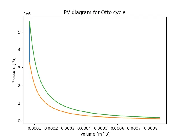
Fig. 1: Plot of PV diagram for Otto cycle

4. Discussion

The evaluation of pressure and volume values for the different stages of a four-stroke engine and especially using a range of different values for starting and ending crank angle during the compression and expansion strokes, as was observed in the concerned plot, greatly assisted in visualising the engine kinematics and estimating the thermal efficiency. The different processes involved as seen in the PV diagram include the first adiabatic process wherein the piston moves in a direction so as to compress the fuel-air mixture leading to slight increase in pressure and temperature without heat being exchanged. Combustion is initiated as soon as the fuel makes contact with the spark plug being ignited. During combustion, the chamber becomes highly pressurized containing a lot of thermal energy and is also identified as an isochoric process. The consequence of the generated thermal energy is that it is directed to do work on the piston thereby moving it back to its location before compression resulting in an increase in the volume of the chamber. This stage is also known as the expansion stage or power stroke as thermal energy is used to create motion to power the machine or vehicle. The last stage is known as the exhaust phase and heat during this stage leaves the gas leading to decrease in pressure.

5. Conclusion

Calculation of kinematics and thermal efficiency of a four-stroke engine implemented across a range of different values for crank angles between 0 and 180 degrees during compression and expansion strokes in Python using the Sublime Text source code editor was well understood with this programming exercise. It was realised that pressure and volume changes during the different stages in a four-stroke engine allowed for key insights to be gained in terms of understanding the nature of the processes involved along with a visual representation in the form of the concerned plot, and that they serve as important aids in improving the design parameters of such engines with focus also being on improving the overall efficiency.

References

[1] NASA, Specific Heats Cp and Cv, www.grc.nasa.gov, viewed 08 December 2021, Specific Heats Cp and Cv

CODE:

Program to calculate the kinematics and thermal efficiency of a four-stroke engine and create its PV diagram.

# Program to calculate the engine kinematics and the thermal efficiency of the engine, and create a PV diagram
# Author: Diptesh Pawa

# Modules/Libraries
import math
import matplotlib.pyplot as plt

# Function to calculate volume based on engine characteristics and crank angle
def engine_kinematics(bore, stroke, con_rod, c_r, start_crank, end_crack):
	a = stroke/2 							# Crank pin radius [m]
	R = con_rod/a							# Constant term

	sc = math.radians(start_crank)			# Starting Crank Angle
	ec = math.radians(end_crack)			# Ending Crank Angle
	num_values_sc_ec = 50
	dtheta = (ec-sc)/(num_values_sc_ec-1)
	V = []

	for i in range(0,num_values_sc_ec):
	 	theta = sc + i*dtheta 
	 	term_1 = 0.5*(c_r-1)
	 	term_2 = R + 1 - math.cos(theta)
	 	term_3 = pow((pow(R,2) - pow(math.sin(theta),2)),0.5)

	 	V.append((1 + term_1*(term_2 - term_3))*V_c)

	return V

# Inputs
# Engine Characteristics
bore = 0.1 									 # Cylinder bore diameter [m]		
stroke = 0.1								 # Stroke Length [m]
con_rod = 0.15								 # Length of connecting rod [m]
c_r = 12 									 # Compression ratio [-]

# State variables and specific heat of air
P_1 = 101325								 # Pressure at state 1 [Pa]
T_1 = 500									 # Temperature at state 1 [K]
gamma = 1.4									 # Specific heat of air
T_3 = 2300									 # Temperature at state 3 [K]

# Outputs
# Volume computations
V_s = math.pi*(1/4)*pow(bore,2)*stroke  	 # Stroke volume [m^3]
V_c = V_s/(c_r-1)  							 # Compression volume [m^3]
V_1 = V_s + V_c								 # Volume at state 1 [m^3]
V_2 = V_c									 # Volume at state 2 [m^3]

# Pressure and temperature computations at state 2
P_2 = (P_1*pow(V_1,gamma))/(pow(V_2,gamma))  # Relation: P_1.V_1^γ = P_2.V_2^γ 
T_2 = ((P_2*V_2)/(P_1*V_1))*T_1  			 # Relation: P_1.V_1/T_1 = P_2.V_2/T_2

# Volume and pressure computations for compression
V_compression = engine_kinematics(bore, stroke, con_rod, c_r, 180, 0)
constant = P_1*pow(V_1,gamma)
P_compression = []
for v in V_compression:
	P_compression.append(constant/pow(v,gamma))

# Volume and Pressure computations at state 3
V_3 = V_2
P_3 = (P_2*V_2*T_3)/(V_3*T_2)  			 	 # Relation: P_2.V_2/T_2 = P_3.V_3/T_3

# Volume and pressure computations for expansion
V_expansion = engine_kinematics(bore, stroke, con_rod, c_r, 0, 180)
constant = P_3*pow(V_3,gamma)
P_expansion = []
for v in V_expansion:
	P_expansion.append(constant/pow(v,gamma))

# Volume, Pressure and Temperature computations at state 4
V_4 = V_1
P_4 = (P_3*pow(V_3,gamma))/(pow(V_4,gamma))  # Relation: P_3.V_3^γ = P_4.V_4^γ
T_4 = ((P_4*V_4)/(P_3*V_3))*T_3  			 # Relation: P_3.V_3/T_3 = P_4.V_4/T_4

# Thermal efficiency of the engine
eta_otto = 1 - (1/(pow(c_r,gamma-1)))
print(eta_otto)

# Plotting of P-V cycle
plt.plot([V_2,V_3],[P_2,P_3])
plt.plot(V_compression,P_compression)
plt.plot(V_expansion,P_expansion)
plt.plot([V_4,V_1],[P_4,P_1])
plt.xlabel('Volume [m^3]')
plt.ylabel('Pressure [Pa]')
plt.title("PV diagram for Otto cycle")
plt.savefig('Week_2_Air_standard_Cycle.png')
plt.show()