Week 8 - Simulation of a backward facing step in OpenFOAM
1. Introduction
The backward facing step geometry is a classical example that offers insight into the phenomena of separating and attaching flows otherwise commonly observed in aerodynamic applications like flow over airfoil and diffusers to name a few. The aim of this challenge is to perform two-dimensional transient numerical simulations of an incompressible-laminar-viscous flow through the backward facing step geometry wherein the grading factor defining all the hex blocks for the given computational domain remain unchanged i.e., GF =1, while in another setup, the grading factor changes to 0.2 such that cells are finer near the walls, including at the step wall.
2. Method
The typical approach adopted to performing numerical simulation in OpenFOAM involves the following steps:
- Identifying the tutorial in the 'FOAM_TUTORIALS' folder that contains the appropriate governing equations relevant to the physics of the flow for the given problem. A typical file structure of an OpenFOAM tutorial consists of the below mentioned directories and files:
- A 'system' directory with the 'controlDict', 'fvSchemes' and 'fvSolution' files used for specifying the numerical schemes and solution procedure along with control on the simulation run properties. Additionally, for the given numerical problem, a file by the name 'blockMeshDict' mentions the creation of different blocks representing the geometry as well as its mesh properties.
- A 'constant' directory that contains a 'polyMesh' directory outlining the various aspects of the mesh such as 'boundary', 'points', 'faces', etc., and a file that defines the physical properties, in this case, 'transportProperties' specifying the value of kinematic viscosity.
- A time directory, usually called the '0' directory that consists of files representing the different fields or fluid flow properties with values as required at the start of simulation run or at time `t = 0`.
- Copying the now identified tutorial folder from the 'FOAM_TUTORIALS' folder to the 'FOAM_RUN' folder, specifically created to allow simulation run of OpenFOAM numerical simulation cases, with either the same name or preferably a name relevant to the geometry to be discretized.
- Replacing the geometry and boundary list of the pre-existing tutorial with the geometry and boundary list pertaining to the given problem and defining mesh parameters with regards to the flow physics, in this case by updating the 'blockMeshDict' file (Section 2.1 Modelling).
- Updating the fields' files present inside the '0' directory viz., 'U' and 'p', with the boundary list as specified in the 'blockMeshDict' file and appropriate values at the relevant boundary to ensure the given numerical problem has the right boundary conditions and that the solution would be correctly initialised (Section 2.2 Boundary Conditions).
- Updating the 'controlDict' file, in this case the 'deltaT' and 'endTime' parameters with values that take into consideration domain specific attributes such as length of the domain in the direction of flow, fluid flow velocity and avoiding violation of Courant-Friedrichs-Lewy Condition or the CFL number by limiting its mean and maximum value during simulation run below 1 (Section 2.4 Determination of transient parameters).
The above steps were executed using Linux commands in a Ubuntu 20.04.2.0 LTS (Long Term Support) operating system as shown below:
i) Change directory to FOAM_RUN:
cd $FOAM_RUN
ii) Copy cavity example from FOAM_TUTORIALS directory that contains the icoFoam solver to the FOAM_RUN directory:
cp -r $FOAM_TUTORIALS/incompressible/icoFoam/cavity/cavity .
iii) Rename cavity directory to Week_8_backward_facing_step_geometry_GF_1 (for performing numerical simulations on backward facing step geometry without using any grading factor (i.e., GF = 1))
mv cavity Week_8_backward_facing_step_geometry_GF_1
iv) Change directory to Week_8_backward_facing_step_geometry_GF_1:
cd Week_8_backward_facing_step_geometry_GF_1
v) Replacing the geometry and boundary list by editing the 'blockMeshDict' file:
gedit system/blockMeshDict
vi) Updating the boundary list and boundary conditions by editing the 'U' and 'p' files:
gedit 0/U
gedit 0/p
vii) Updating the 'deltaT' and 'endTime' parameters with appropriate values by editing the 'controlDict' file:
gedit system/controlDict
viii) Creating the block based geometry and generating mesh for the computational domain:
blockMesh
ix) Running the icoFoam solver to solve for the incompressible laminar Navier-Stokes equations:
icoFoam
x) Post-processing and visualising results of the performed simulation (Section 2.5):
paraFoam
Similarly, a copy of the cavity tutorial was created for performing numerical simulation of backward facing step geometry with grading factor of 0.2 and 5 such that cells are finer near the walls (including at the step wall) by repeating steps i) to x) only this time the folder is renamed in step iii) to 'Week_8_backward_facing_step_geometry_GF_0.2' and directory is changed in step iv) to this newly renamed folder.
2.1 Modelling
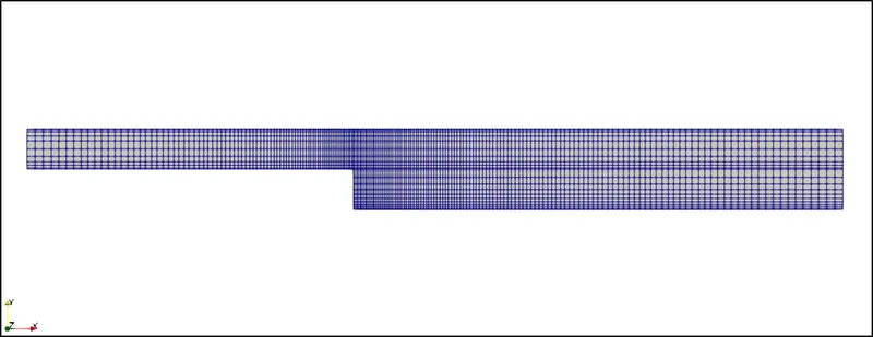
The problem was solved by constructing a set of five three-dimensional hexahedral blocks (number of mesh elements in z-direction was set to 1 implying a two-dimensional flow problem) that together resembled the backward facing step geometry (as seen in Fig. 2) with each block defined using 8 vertices in a dictionary type file called 'blockMeshDict' (file snippet for which is attached below with this report). Alignment of the hexahedral blocks were positioned in such a manner that the inlet section of the geometry upto the step were split mid-way along the local y-axis direction creating two hex blocks each of length 0.08m, in the direction of flow, that also continued from the step to the outlet adding two more hex blocks of lengths 0.12m each, also in the direction of flow, while the region constituting the length of the entire step, along the local y-axis direction, to the outlet formed the last or fifth hex block. Vertices were assigned, as seen in Fig. 2, representing the 8 corners at each hexahedron block in which the origin, or point '0', was selected as the first point on the back face in hex block '1' along the flow direction. The line stating the creation of hex blocks in the 'blockMeshDict' file followed the arrangement of vertices according to the right-hand system such that the normal (direction in which the thumb of the right hand pointed towards) was oriented outwards for the plane containing vertices 11, 12, 13, 14, 15, 16, 17, 18, 19, 20 and 21, outlining the extents of the blocks to the viewer implying the vertices were to be numbered along which the remaining fingers of the right hand curled towards, i.e., in counter-clockwise direction. The principle remained the same for defining the faces of the boundaries in the 'boundary' section of the 'blockMeshDict' file, only this time the normals would face outwards from each of the respective planes such that the region defining the 'inlet' would have its normal facing outwards in the negative x-axis direction, 'outlet' with normal in the positive x-axis direction, top wall surface of the domain with normal in the positive y-axis direction, bottom wall surfaces of the domain with normal in the negative y-axis direction, front surface of the domain with normal in the positive z-axis direction and back surface of the domain with normal in the negative z-axis direction while vertices would be numbered in a similar manner again along the direction in which the remaining fingers of the right hand curled towards for each of the regions mentioned previously. The total number of grid points along both the x-axis and y-axis directions have been so taken such that a cell is created at every 0.001m or in other words, number of cells along the longer x direction is 200 while number of cells along the longer y direction is 20. A hex block definition also consists of specifying the cell expansion ratios, in this case along each local cartesian coordinate direction using 'simpleGrading', which equates to the ratio of the width of the end/last cell to the width of the start/first cell along the same edge of a particular block. A cell expansion ratio of 1 indicates that the width of the end/last cell is equal to the width of the start/first cell i.e., the first case study of the given numerical simulation, while a cell expansion ratio of 0.2 indicates that the width of the end/last cell is equal to 0.2 times the width of the start/first cell and a cell expansion ratio of 5 indicates that the width of the end/last cell is equal to 5 times the width of the start/first cell i.e., the second case study of the given numerical simulation. Grading factor of 0.2 was used in blocks wherein the last cell was positioned near the walls and step wall of the given domain while grading factor of 5 in blocks where the last cell was located far from the walls and step wall, along both the x-axis and y-axis directions, in order to refine the region where the velocity and pressure gradients were likely to vary the most viz., at the surface area change of the domain in the direction of flow and along the walls where the velocity would arrive at 0 due to the no-slip boundary condition.
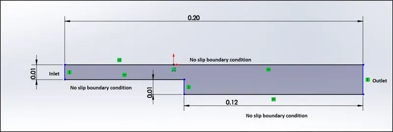
Fig. 1: Backward Facing Step Geometry (Source: Week 8 - Simulation of a backward facing step in OpenFOAM Question)
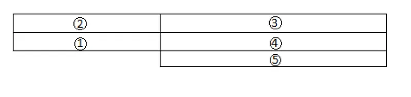
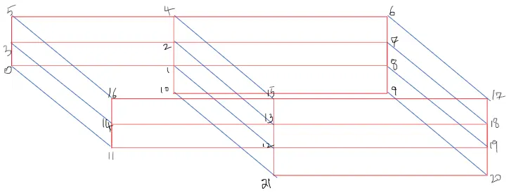
Fig. 2:The five hexahedral blocks and vertices representing the decomposed main domain (Courtesy: Text help for blockMesh)
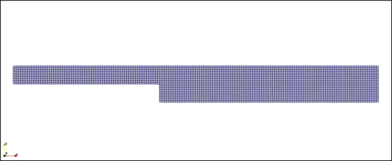
a) b)
Fig. 3: Meshed domain: a) Without using any grading factor (i.e., GF = 1), b) Grading factor of 0.2 such that cells are finer near the walls (including at the step wall).
2.2 Boundary Conditions
The different regions of the mesh, identified as patches, that demarcate its extents as well as specify the boundary conditions to be employed on them is written in a list called as 'boundary' in the 'blockMeshDict' file. The input and output data in OpenFOAM are recorded as tensor fields which are written onto time directories, in this case the fields being velocity ('U') and pressure ('p') in the '0' folder, and read from it at an appropriate time. A typical structure of the field data file consists of the 'dimensions' written with 7 scalars representing the 'dimensionSet' enclosed by square brackets with each scalar highlighting the properties of mass, length, time, temperature, quantity, current and luminous intensity respectively from left to right in base units for SI and USCS, 'internalField', in this case of type 'uniform', that allocates a single value to all elements within the field and expressed using 3 vector components for velocity (U) and only 'uniform 0' for pressure (p) as it is kinematic pressure for an incompressible case for which its absolute value is of little significance, and 'boundaryField' which consists of a list of boundary conditions and data for all patches, preferably identical in name to the patches created in 'boundary' in the 'blockMeshDict' file. For the given numerical simulation, the different patch names and patch types of the 'blockMeshDict' file and boundary fields (type and value) of the time directory files, 'U' and 'p' (file snippets for which is attached below with this report), describing the numerical simulation of an incompressible-laminar-viscous flow through the backward facing step geometry is mentioned in the following table:
|
patch name |
inlet |
outlet |
fixedWalls |
frontAndBack |
|
patch type (in blockMeshDict) |
patch |
patch |
wall |
empty |
|
type (in U) |
fixedValue |
zeroGradient |
noSlip |
empty |
|
value (in U) |
uniform(1 0 0) |
-- |
-- |
-- |
|
type (in p) |
zeroGradient |
fixedValue |
zeroGradient |
empty |
|
value (in p) |
-- |
uniform 0 |
-- |
-- |
Table 1: Boundary Conditions and its setup
Type 'zeroGradient' in '0' time directory files, 'U' and 'p', indicates the normal gradient of that particular field at the relevant patch name is 0, type 'empty' for the 'frontAndBack' patch is used to highlight the front and back planes of the created two-dimensional domain and type 'noSlip' is used to set the velocity of the 'fixedWalls' patch to (0 0 0).
2.3 icoFoam model
The icoFoam solver uses the PISO pressure-velocity coupling algorithm to solve the incompressible laminar Navier-Stokes equations. The Navier-Stokes equations define the fluid flow properties such as velocity, pressure, density, temperature, viscosity, energy, etc., within a given physical domain. Additionally, the Navier-Stokes equations are developed with regards to the laws of conservation that states the net mass flow across a system is zero (Conservation of mass), momentum within the same system (or control volume) is constant (Conservation of momentum). The continuity and momentum equations are mathematically expressed below as:
Continuity equation: `nabla*U = 0`
Momentum equation: `del/(del t)*(u) + nabla*(uotimesu) - nabla*(nu*nablau) = -nabla p` ; where
`u` is velocity (in m/s), and
`p` is kinematic pressure (in `m^2/s^2`)
2.4 Determination of transient parameters
The setup of simulation run time and time-step size for any given computational domain in OpenFOAM is described in the 'controlDict' dictionary file. Typically, the start of any simulation begins at `t = 0`, in which case OpenFOAM is required to read the field values of the '0' directory and therefore 'startFrom' keyword is set to 'startTime' which is in turn set to 0 referring to the '0' directory. The 'endTime' depends on the domain length and the flow velocity, in the direction of flow, such that the fluid medium passes through it at least 10 times to acquire steady state conditions, in the case of laminar flow as a mark of a general rule and also as a recommendation in the OpenFOAM v8 User Guide. Therefore, 'endTime' can be evaluated as shown below:
`endTime = (L/U)*10`; where (Eq. 1)
`L` is the length of the computational domain = 0.2m, and
`U` is the fluid flow velocity = 1m/s
From Eq. 1, we get value of 'endTime' as 2s. Time-step size, 'deltaT' was decided based on the CFL number which is expressed below:
`CFL = (U*Delta t)/(Delta x)`; where (Eq. 2)
`Delta t` is time-step size,
`Delta x` represents the smallest cell size, which in the case of without using any grading factor (i.e., GF = 1) was calculated as the length of the computational domain to the number of mesh elements in the direction of flow, in this case along x-axis direction, i.e.,
`Delta x = L/n_x`; (Eq. 3)
However, the value of `Delta x` in the case of grading factor of 0.2 implied that the smallest cell size would be 0.2 times the value as that determined in the case of without using any grading factor (i.e., GF = 1), i.e.,
`Delta x = (L/n_x)*0.2`; (Eq. 4)
In order to attain temporal accuracy and numerical stability using the 'icoFoam' solver, the CFL criteria was required to be less than 1 and therefore, the values of time-step size were initially determined with the limiting value of the CFL criteria as 1 and tabulated as shown below:
|
Mesh |
`Delta x` (in m) (Eq. 3 and Eq. 4) |
Time-step size (`Delta t`) (in s) (Eq. 2) |
|
Without using any grading factor (i.e., GF = 1) |
0.001 |
0.001 |
|
Grading factor of 0.2 |
0.0002 |
0.0002 |
Table 2: Smallest element size (`Delta x`) and time-step size (`Delta t`) values for meshes without using any grading factor (i.e., GF = 1) and with grading factor of 0.2
The above calculated values of time-step size for both meshes in Table 2 resulted in the mean Courant number to report values less than 1 for mesh without using any grading factor (GF = 1), however, the mean Courant number for mesh with grading factor of 0.2 and maximum Courant number for both meshes continued to be greater than 1. Therefore, the time-step size was further reduced by half its calculated value (as seen in Table 2) for both meshes i.e., for mesh without using any grading factor (GF = 1), the time-step size was altered to 0.0005s, while for mesh with grading factor of 0.2, the time-step size was changed to 0.0001s (file snippet for which is attached below with this report).
2.5 Post-Processing
Plotting the velocity profiles at 0.085 m from the inlet of the geometry was performed by using ParaView's in-built "plot over line" tool. The "plot over line" tool was accessed by clicking on 'Filters' present in the data analysis group, followed by inputting the coordinates as seen in Table 3, and then clicking on the "Apply" button to view the said profile. It was ensured that only the "U" field and time-step as the last time-step size of the simulation run were selected to view the velocity profile results. In order to provide for a better comparison between the velocity profiles of the two numerical simulations i.e., with and without grading, the plot data was extracted to an Excel file by selecting 'Export Scene' option under the 'File' menu in the 'Main Controls' toolbar and providing an appropriate name for the output documents before saving it. Additionally, velocity (U) and pressure (p) field plots were created to view the development of the flow field characteristics across the fluid domain. A legend, title, x label and y label were added for a better understanding of the graphical representation.
|
Line |
x |
y |
z |
|
Point 1 |
0.085 |
-0.01 |
0 |
|
Point 2 |
0.085 |
0.01 |
0 |
Table 3: Line Coordinates for viewing the velocity profiles
3. Results
3.1 Velocity profiles for different meshes (with and without grading)
Fig.4 below shows the velocity profiles computed for different meshes i.e., without any grading factor (GF = 1) and using a grading factor of 0.2 for refinement of cells near the walls (including at the step wall). It can be seen that decreasing the cell size near the walls and step wall regions, the shape of the profile tends towards a more narrow curved peak region as compared to the grid that has an even distribution of cells across the entire domain. This can be attributed to the fact that the gradients of velocity along the direction of flow and especially in the vicinity of the walls and step wall zones vary more drastically and is better captured with smaller element sizes, in this case with grading factor of 0.2. The differences seem to be less noticeable while viewing the field plots i.e., for velocity (U) and pressure (p) between the two previously mentioned meshes as the development of the flow fields are almost similar and therefore only single plots (Fig. 5) of the computational domain were included for visualization for the case of without any grading factor (GF = 1).
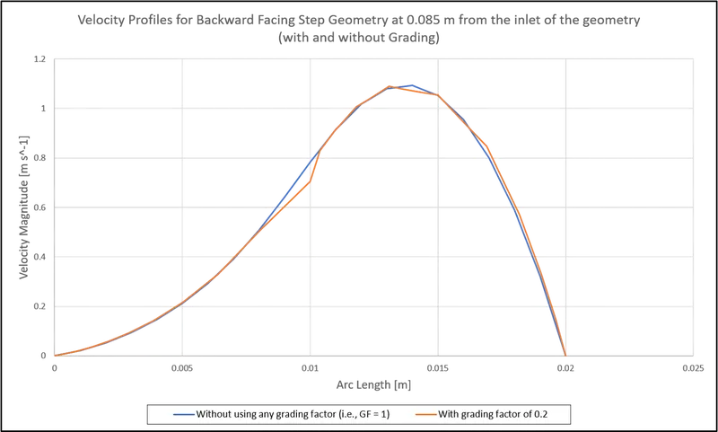
Fig. 4: Plot of Velocity Profile at 0.085 m from the inlet of the Backward Facing Step geometry (with and without Grading)
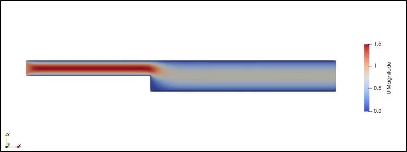
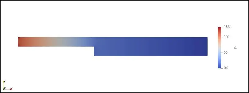
Fig. 5: Velocity and Pressure field plots across the Backward Facing Step geometry for domain without using any grading factor (i.e., GF = 1)
4. Discussion
The evaluation of velocity profiles for the two different meshes indicates the significance of grading/growth factor as the mesh without any grading factor (GF = 1) was not refined enough to capture the near wall gradients of the flow properties, especially velocity, as compared to the mesh using a grading factor of 0.2 in the relevant blocks of the decomposed domain. This implies that the computational model developed without any grading factor, for the given numerical problem, would be less reliable and less accurate in comparison to its experimental model as well as have more errors due to the presence of increased numerical diffusion than the computational model using appropriate grading factor that better captures the physics of the flow.
5. Conclusion
The numerical simulation of a backward facing step geometry using the blockMesh and icoFoam commands to execute the 'blockMeshDict' file for creating the geometry and meshed computational domain, and solving the incompressible laminar Navier-Stokes equations respectively in OpenFOAM was well understood. It was realised that based on the values of grading factor, and time-step size and total time, the resulting velocity profiles could be made to assume a shape more attuned with the physics of the flow as that would be determined from experimental studies in conjunction with a steady-state solution and limiting the possibilities of violation of CFL number.
Dictionary and Fields Files:
1. blockMeshDict file [Without using any grading factor (i.e., GF = 1)]
/*--------------------------------*- C++ -*----------------------------------*
  =========                 |
  \      /  F ield         | OpenFOAM: The Open Source CFD Toolbox
   \    /   O peration     | Website:  https://openfoam.org
    \  /    A nd           | Version:  8
     \/     M anipulation  |
*---------------------------------------------------------------------------*/
FoamFile
{
    version     2.0;
    format      ascii;
    class       dictionary;
    object      blockMeshDict;
}
// * * * * * * * * * * * * * * * * * * * * * * * * * * * * * * * * * * * * * //

convertToMeters 1;

vertices
(
    (0 0 0)
    (0.08 0 0)
    (0.08 0.005 0)
    (0 0.005 0)
    (0.08 0.01 0)
    (0 0.01 0)
    (0.20 0.01 0)
    (0.20 0.005 0)
    (0.20 0 0)
    (0.20 -0.01 0)
    (0.08 -0.01 0)
    (0 0 0.1)
    (0.08 0 0.1)
    (0.08 0.005 0.1)
    (0 0.005 0.1)
    (0.08 0.01 0.1)
    (0 0.01 0.1)
    (0.20 0.01 0.1)
    (0.20 0.005 0.1)
    (0.20 0 0.1)
    (0.20 -0.01 0.1)
    (0.08 -0.01 0.1)
);

blocks
(
    hex (0 1 2 3 11 12 13 14) (80 5 1) simpleGrading (1 1 1)
    hex (3 2 4 5 14 13 15 16) (80 5 1) simpleGrading (1 1 1)
    hex (2 7 6 4 13 18 17 15) (120 5 1) simpleGrading (1 1 1)
    hex (1 8 7 2 12 19 18 13) (120 5 1) simpleGrading (1 1 1)
    hex (10 9 8 1 21 20 19 12) (120 10 1) simpleGrading (1 1 1)
);

edges
(
);

boundary
(
    inlet
    {
        type patch;
        faces
        (
            (0 11 14 3)
            (3 14 16 5)
        );
    }
    outlet
    {
        type patch;
        faces
        (
            (9 8 19 20)
            (8 7 18 19)
            (7 6 17 18)
        );
    }
    fixedWalls
    {
        type wall;
        faces
        (
            (16 15 4 5)
            (15 17 6 4)
            (0 1 12 11)
            (21 10 9 20)
            (10 21 12 1)
        );
    }
    frontAndBack
    {
        type empty;
        faces
        (
            (0 3 2 1)
            (3 5 4 2)
            (10 1 8 9)
            (1 2 7 8)
            (2 4 6 7)
            (11 12 13 14)
            (14 13 15 16)
            (13 18 17 15)
            (12 19 18 13)
            (21 20 19 12)
        );
    }
);

mergePatchPairs
(
);

// ************************************************************************* //
2. blockMeshDict file [Grading factor of 0.2 and 5 such that cells are finer near the walls (including at the step wall)]
/*--------------------------------*- C++ -*----------------------------------*
  =========                 |
  \      /  F ield         | OpenFOAM: The Open Source CFD Toolbox
   \    /   O peration     | Website:  https://openfoam.org
    \  /    A nd           | Version:  8
     \/     M anipulation  |
*---------------------------------------------------------------------------*/
FoamFile
{
    version     2.0;
    format      ascii;
    class       dictionary;
    object      blockMeshDict;
}
// * * * * * * * * * * * * * * * * * * * * * * * * * * * * * * * * * * * * * //

convertToMeters 1;

vertices
(
    (0 0 0)
    (0.08 0 0)
    (0.08 0.005 0)
    (0 0.005 0)
    (0.08 0.01 0)
    (0 0.01 0)
    (0.20 0.01 0)
    (0.20 0.005 0)
    (0.20 0 0)
    (0.20 -0.01 0)
    (0.08 -0.01 0)
    (0 0 0.1)
    (0.08 0 0.1)
    (0.08 0.005 0.1)
    (0 0.005 0.1)
    (0.08 0.01 0.1)
    (0 0.01 0.1)
    (0.20 0.01 0.1)
    (0.20 0.005 0.1)
    (0.20 0 0.1)
    (0.20 -0.01 0.1)
    (0.08 -0.01 0.1)
);

blocks
(
    hex (0 1 2 3 11 12 13 14) (80 5 1) simpleGrading (0.2 5 1)
    hex (3 2 4 5 14 13 15 16) (80 5 1) simpleGrading (0.2 0.2 1)
    hex (2 7 6 4 13 18 17 15) (120 5 1) simpleGrading (5 0.2 1)
    hex (1 8 7 2 12 19 18 13) (120 5 1) simpleGrading (5 5 1)
    hex (10 9 8 1 21 20 19 12) (120 10 1) simpleGrading (5 5 1)
);

edges
(
);

boundary
(
    inlet
    {
        type patch;
        faces
        (
            (0 11 14 3)
            (3 14 16 5)
        );
    }
    outlet
    {
        type patch;
        faces
        (
            (9 8 19 20)
            (8 7 18 19)
            (7 6 17 18)
        );
    }
    fixedWalls
    {
        type wall;
        faces
        (
            (16 15 4 5)
            (15 17 6 4)
            (0 1 12 11)
            (21 10 9 20)
            (10 21 12 1)
        );
    }
    frontAndBack
    {
        type empty;
        faces
        (
            (0 3 2 1)
            (3 5 4 2)
            (10 1 8 9)
            (1 2 7 8)
            (2 4 6 7)
            (11 12 13 14)
            (14 13 15 16)
            (13 18 17 15)
            (12 19 18 13)
            (21 20 19 12)
        );
    }
);

mergePatchPairs
(
);

// ************************************************************************* //
3. Velocity (U) field file
/*--------------------------------*- C++ -*----------------------------------*
  =========                 |
  \      /  F ield         | OpenFOAM: The Open Source CFD Toolbox
   \    /   O peration     | Website:  https://openfoam.org
    \  /    A nd           | Version:  8
     \/     M anipulation  |
*---------------------------------------------------------------------------*/
FoamFile
{
    version     2.0;
    format      ascii;
    class       volVectorField;
    object      U;
}
// * * * * * * * * * * * * * * * * * * * * * * * * * * * * * * * * * * * * * //

dimensions      [0 1 -1 0 0 0 0];

internalField   uniform (0 0 0);

boundaryField
{
    inlet
    {
        type            fixedValue;
        value           uniform (1 0 0);
    }

    outlet
    {
        type            zeroGradient;
    }

    fixedWalls
    {
        type            noSlip;
    }

    frontAndBack
    {
        type            empty;
    }
}

// ************************************************************************* //
4. Pressure (p) field file
/*--------------------------------*- C++ -*----------------------------------*
  =========                 |
  \      /  F ield         | OpenFOAM: The Open Source CFD Toolbox
   \    /   O peration     | Website:  https://openfoam.org
    \  /    A nd           | Version:  8
     \/     M anipulation  |
*---------------------------------------------------------------------------*/
FoamFile
{
    version     2.0;
    format      ascii;
    class       volScalarField;
    object      p;
}
// * * * * * * * * * * * * * * * * * * * * * * * * * * * * * * * * * * * * * //

dimensions      [0 2 -2 0 0 0 0];

internalField   uniform 0;

boundaryField
{
    inlet
    {
        type            zeroGradient;
    }

    outlet
    {
        type            fixedValue;
        value           uniform 0;
    }

    fixedWalls
    {
        type            zeroGradient;
    }

    frontAndBack
    {
        type            empty;
    }
}

// ************************************************************************* //
5. controlDict file [for blockMeshDict file without using any grading factor (i.e., GF = 1)]
/*--------------------------------*- C++ -*----------------------------------*
  =========                 |
  \      /  F ield         | OpenFOAM: The Open Source CFD Toolbox
   \    /   O peration     | Website:  https://openfoam.org
    \  /    A nd           | Version:  8
     \/     M anipulation  |
*---------------------------------------------------------------------------*/
FoamFile
{
    version     2.0;
    format      ascii;
    class       dictionary;
    location    "system";
    object      controlDict;
}
// * * * * * * * * * * * * * * * * * * * * * * * * * * * * * * * * * * * * * //

application     icoFoam;

startFrom       startTime;

startTime       0;

stopAt          endTime;

endTime         2;

deltaT          0.0005;

writeControl    timeStep;

writeInterval   20;

purgeWrite      0;

writeFormat     ascii;

writePrecision  6;

writeCompression off;

timeFormat      general;

timePrecision   6;

runTimeModifiable true;


// ************************************************************************* //
6. controlDict file [for blockMeshDict file with grading factor of 0.2 and 5 such that cells are finer near the walls (including at the step wall)]
/*--------------------------------*- C++ -*----------------------------------*
  =========                 |
  \      /  F ield         | OpenFOAM: The Open Source CFD Toolbox
   \    /   O peration     | Website:  https://openfoam.org
    \  /    A nd           | Version:  8
     \/     M anipulation  |
*---------------------------------------------------------------------------*/
FoamFile
{
    version     2.0;
    format      ascii;
    class       dictionary;
    location    "system";
    object      controlDict;
}
// * * * * * * * * * * * * * * * * * * * * * * * * * * * * * * * * * * * * * //

application     icoFoam;

startFrom       startTime;

startTime       0;

stopAt          endTime;

endTime         2;

deltaT          0.0001;

writeControl    timeStep;

writeInterval   20;

purgeWrite      0;

writeFormat     ascii;

writePrecision  6;

writeCompression off;

timeFormat      general;

timePrecision   6;

runTimeModifiable true;


// ************************************************************************* //