Rayleigh Taylor Instability Challenge

1. Introduction

The hydrodynamic instability caused as a result of having a heavy fluid (or more dense fluid) placed above a light fluid (or less dense fluid) in the presence of the gravitational field leading to the latter fluid trying to push onto the former fluid can be described as the Rayleigh-Taylor Instability (RTI) phenomena after Lord Rayleigh who first investigated and analysed the problem for inviscid fluids with different stratification profiles and G.I. Taylor showed similarities to a problem wherein the interface was accelerated towards the more dense fluid. The RTI phenomena occurs across varying situations ranging from the formation of high luminosity twin exhaust jets observed in gas clouds that are rotating under the influence of an external gravitational potential to laser based implosions of deuterium-tritium fusion targets in a nuclear reactor setup as examples in nature and technological driven applications respectively. The RTI phenomena has many different stages of development and depending on the properties of the concerned fluids, additional challenges are posed in terms of predicting the overall behaviour. Many practical CFD models have been developed to understand the RTI phenomena depending on the prevailing conditions and characteristics to be observed which also includes level set method, volume of fluid (VOF) method and two-phase flow model as examples. The level set method makes use of the level set function which assigns a signed distance to the fluids involved with zero value representing the interface position thereby allowing accurate calculations of spatial gradients due to the smooth and continuous definition of the said function which is useful for tracking in two phase flows for topologically complicated interfaces with the added benefit of accounting for surface tension effects caused as a result of curvature around the interface region. The only associated drawback with the level set method is that volume conservation preservation is prone to deficiency. The VOF method, on the other hand, is also a surface tracking technique with the distinction that the volume conservation is naturally preserved as the computation and tracking of the volume fraction of a particular phase occurs in each cell rather than at the interface, however, because of the definition of the VOF function, calculation of spatial derivatives is discontinuous. Both the level set method and the VOF method are models categorised under the Euler-Euler approach with the different phases involved being mathematically treated as interpenetrating continua. Based on real world situations as was observed by Youngs [1], instabilities propagate as a result of multiple initial wavelength perturbations leading to turbulent mixing within the given media. This information coupled with experimental investigations lead to the development of the two-phase flow model based on the two-fluid turbulence model that was utilised by Spalding. The multiphase model accommodates the effects of differential acceleration as a result of the underlying pressure gradients on fluid fragments of different densities, drag between fluid fragments, additional mass, increase in length scale of the bubble or drop radius in proportion to the width of the mixing region as well as the extra effects of inter-fluid drag that promotes mixing in the form of turbulence kinetic energy equation, mass and momentum transport by turbulent diffusion and length scale diffusion [2].

The aim of this challenge is to perform transient simulations using the laminar viscous and the VOF Multiphase model in ANSYS Fluent 2020 R1 to understand the RTI phenomena through its different stages of development. Analysis of the RTI phenomena is performed between two different mesh sizes for Air and Water as materials representing the two different phases to understand the impact of mesh density as well as comparing the development process for the more refined mesh with Water and a user-defined material. The meshes prepared highlight the mesh quality attributes like element quality, skewness, orthogonality and aspect ratio apart from the cell count, volume fraction for water and number of iterations for convergence for each mesh based on stability of behaviour of the volume fraction for water values. Additional investigations would also be carried out on the Atwood number, which represents a dimensionless quantity as the ratio of the difference in the fluid densities to the sum of the same, and the manner in which it plays a role with regards to the RTI phenomena.

2. Method

2.1 Modelling

The computational domain for simulating the RTI phenomena was modelled in SpaceClaim, the default solid modeling CAD software for the Fluid Flow (Fluent) Analysis System, in a two-dimensional space. The individual sub-domains representing phases for two different materials were each created with dimensions of 20mm indicating the length and width measurement values while ensuring that the sub-domains shared the same common interface. This was possible by drawing the extents of one sub-domain and using the same plane to sketch the other sub-domain. SpaceClaim offers a feature called the 'Pull' tool in the 'Edit' menu of the 'Design' tab which will highlight the independent sub-domains during their creation by changing the colour indicating that the surface has been created. The sub-domains were moved to their independent components by right-clicking on the surface for the first sub-domain and then the parent model structure tree for the remaining one. For creating a mesh wherein the nodes on both sides of the interface in the mesh match, or in other words is conformal, both the surfaces representing the individual sub-domains were selected and the 'Share Prep' button available in the 'Sharing' section under the 'Workbench' tab was clicked on. By enabling this feature, the exchange of information across the independent sub-domains was allowed which would offer negligible to minimum interpolation especially at the interface thereby improving computational time and rendering higher accuracy to the solution.

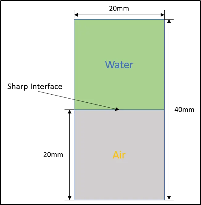
Fig. 1: Fluid Volume Model

2.2 Meshing

The meshing approach adopted for the given computational domain was developed to maintain the meshing quality attributes viz., element quality, skewness, orthogonality and aspect ratio within the ranges as laid out in the Meshing training material of ANSYS outlined in the following table:

Element Quality			0 (Bad Mesh)	1 (Good Mesh)
Aspect Ratio		Triangles	1 (for an equilateral triangle)	- Best possible value
		Quadrilaterals	1 (for a square)	- Best possible value
Skewness	0-0.25 (Excellent)	0.25-0.50 (Very Good)	0.50-0.80 (Good)	0.80-0.94 (Acceptable)	0.95-0.97 (Bad)	0.98-1.00 (Unacceptable)
Orthogonal Quality	0-0.001 (Unacceptable)	0.001-0.14 (Bad)	0.15-0.20 (Acceptable)	0.20-0.69 (Good)	0.70-0.95 (Very Good)	0.95-1.00 (Excellent)

Table 1: Mesh Quality Attributes as defined in the ANSYS meshing training material

The reason for targeting the above mentioned mesh quality attributes comes from analysis across different types of geometries/models that these are few of the known ways of identifying whether the discretized mesh would develop convergence issues during the solution process and also to locate areas in the mesh where the statistics can be improved. In Section 2.4.1 and Section 2.4.2, we will discuss about both the Baseline mesh and the Refined mesh that were prepared as well as their qualities.

2.3 CFD Simulation Setup, Material Definition, Monitoring Report setup and Solution

The simulations on all meshes was performed using the Laminar viscous and the VOF Multiphase models. For the given modelling configuration, the multiphase flow regime represents that of a stratified/free-surface flow identified as a result of the flow of immiscible fluids separated by a distinctly clear interface. Based on the clarity of the multiphase flow regime and the fact that the interface position (or subsequent collapse) is the topic of interest, the VOF Multiphase model is best suited for the given numerical analysis. Additionally, all simulations are being run using the double-precision feature to accurately measure the prediction quantities (volume fraction of water) and as a general measure to resolve large variations in pressure differences. A brief description into the working of the Laminar viscous and the VOF Multiphase models is provided below:

2.3.1 Laminar viscous model

The Laminar viscous model can be described as the solution of the governing fluid equation viz., Navier-Stokes equations for a domain, in this case, discretized using the finite volume approach, without the presence of turbulence terms. The Navier-Stokes equations define the fluid flow properties such as velocity, pressure, density, temperature, viscosity, energy, etc., within a given physical domain. Additionally, the Navier-Stokes equations are developed with regards to the laws of conservation that states the net mass flow across a system is zero (Conservation of mass) and that the momentum within the same system (or control volume) is constant (Conservation of momentum). If energy is also a variable of assessment for the given domain, then according to the first law of thermodynamics, total heat gain of a system is equal to the sum of heat added to the system and work done on the same system.

For the given problem, the computational domain is two-dimensional and energy is not a variable of assessment. This implies that the Navier-Stokes equations that will be solved using the Laminar viscous model is for the conservation of mass or continuity equation and conservation of momentum.

2.3.1.1 Setup of the Laminar viscous model:

To use the Laminar viscous model in the Fluent component system, we navigate to Viscous option in Models under the Physics Tab. In the Viscous Model feature window, we choose Laminar as the option.

2.3.2 VOF Multiphase model

The VOF model as mentioned before is a surface-tracking technique employed when flow takes places between two immiscible fluids separated by an interface. The model makes use of a single set of momentum equations, shared by the fluids, with the volume fraction of each fluid computed and tracked in individual cells throughout the domain. The VOF formulation assigns a variable in the form of volume fraction of phases depending on the number of phases involved such that the sum of volume fractions of all phases equals to unity and also that the phases involved are not interpenetrating. This subsequently also leads to the respective fields for all variables and properties to be shared by the phases thereby creating volume-averaged values depending on the volume fraction of each phase at a given location.

2.3.2.1 Setup of the VOF Multiphase model

To use the VOF model in the Fluent component system, we navigate to Multiphase option in Models under the Physics Tab. In the Multiphase Model window, we choose Volume of Fluid under Homogeneous Models, Implicit Formulation under Volume Fraction Parameters and Sharp Type as Options for Interface Modeling as the setup configuration. It should be noted that Volume of Fluid model is only available under the Homogeneous Models section which implies that the phases in the domain are assumed to move with the same velocity, as is commonly assumed for free surface flows, and that all phases share all of the field variables except for volume fraction.

2.3.3 Material Definition and Monitoring Report setup

For the given problem, the material properties representing individual sub-domains include Air with Density value of 1.225 `(kg)/m^3`, Viscosity (or dynamic viscosity) value of `1.7894*10^(-5) (kg)/(ms)`, Water with Density value of 998.2 `(kg)/m^3`, Viscosity (or dynamic viscosity) value of `0.001003 (kg)/(ms)` and user-defined material with Density value of 400 `(kg)/m^3` and Viscosity (or dynamic viscosity) value of `0.001 (kg)/(ms)`. The materials Air, Water and user-defined material can be verified by heading over to the "fff-air-surface" zone for the first and the last material definitions and "fff-water_surface" zone for the second material definition of "Cell Zones" under the "Zones" section of the "Physics" tab and click on "Edit" button for viewing the different attributes of the same. While Air and Water material definitions would be allocated to the respective zones by Fluent itself (in most cases), user-defined material needs to be created first which can be done by clicking on the 'Create/Edit Materials' in the same options list as the "Cell Zones" and entering the values for "Density" and "Viscosity" provided in the problem statement with Air as the selected material while ensuring that the properties of Air are not overridden when the "Change/Create" button in the 'Create/Edit Materials' window is clicked on. The resulting action will create a copy of the user-defined material which can then be chosen as the preferred material for the "fff-air-surface" zone in "Cell Zones" and thereafter Air can be removed from the material list to avoid ambiguity. The material definition allows for easier allocation of the "Primary Phase" and "Secondary Phase" as the required "Phases" during the "Phase Setup" process available under the "Phases" tab in the Multiphase Model window with either Air or the user-defined material representing the "Primary Phase" and Water as the "Secondary Phase".

During the solution process, we are interested in monitoring the volume fraction for water plot across the entire domain to observe the flow behaviour. To create the required monitoring plot, we head over to the 'Definitions' drop-down menu in the 'Reports' section of the 'Solution' tab and choose 'Area-Weighted Average' option in the 'Surface Report' followed by assigning the name as vof-water, choosing 'Phases' as the Field Variable and 'Volume fraction' as the attribute with the 'Phase' set to Water, selecting all surfaces in the 'Surfaces' list, checking the 'Report File' and 'Report Plot' boxes before clicking on the 'OK' button.

2.3.4 Solution

The nature of given CFD simulation is transient while type of solver chosen is Pressure-based solver as we are dealing with a low-speed incompressible flow problem i.e., speed of fluid flow is typically in the subsonic range and density of material does not change or the change is almost negligible within the given control volume, although the Fluent Theory Guide also claims that the Pressure-based solver can now solve and operate beyond its previous limitations. A steady-state VOF calculation is not possible for the given numerical analysis as there are no inflow boundaries for the individual phases as well as the resulting solution is not independent of initial conditions which in this case is the initial level of fluid in both individual sub-domains. The Pressure-based solver calculates the Pressure field by evaluating the pressure or pressure-correction equation that is determined from the manipulation of continuity and momentum equations. Velocity formulation is chosen to be absolute as the velocity in the given fluid control volume is not rotating. Since, the RTI phenomena was being studied under the influence of the gravitational field, 'Gravity' option was enabled with y-axis as the reference direction and value in Y set to -9.81 `m/(s^2)` representing downward direction of gravitational acceleration on the system. Before the solution was run, we initialised the given fluid volume which in this case was done using the Standard Initialisation option. Standard Initialisation as described in the Fluent Theory Guide allows the user to specify all the variables directly as initial guess values across each cell of the entire domain. The variables can include initial guess values for velocity, temperature, pressure, etc. from the available list. In the given computational analysis, the use of Standard Initialisation was combined with Patch option to assign the volume fraction values to Water phase as 1 and Air phase as 0. A contour plot to depict the collapse of the interface as a function of time as part of the development of the RTI phenomena during the simulation run and recorded as a MPEG animation file was setup. The contour plot was now available to be created under the 'Graphics' section of the 'Results' tab since the solution was initialized. After a new contour plot option was selected from the 'Contours' drop-down menu, a name was assigned, in this case, 'vof-water-RTI', followed by clicking on the 'Filled' check-box, choosing 'Phases' as the field variable with 'Volume Fraction' as the attribute, setting 'Phase' to Water and selecting all the surfaces in the 'Surfaces' list before clicking on the 'Save/Display' button. An animation plot of the same contour was created by heading back to the 'Solution' tab and clicking on the 'Solution Animations' option available under the 'Create' drop-down menu of the 'Activities' section. In the 'Animation Definition' window, the name of the animation was assigned as 'vof-water-RTI-animation' and 'vof-water-RTI' was chosen which was the name of the contour plot before clicking on 'OK'. Additionally, during the entire run, the default convergence criteria values were unaltered for 'continuity', 'x-velocity', 'y-velocity', and 'vf-water' as tabulated in Table 6. The definition of run calculation activities were based around the time step size, number of time steps and maximum iterations per time step. Due to challenges in estimating the growth rate of the RTI phenomena based on the propagation of the growing perturbations around the interface as a result of insufficient information about the wavelength combined with formation of different structures like spikes, bubbles, mushrooms, etc., a rough analogy based on the maximum possible velocity in the given domain was calculated as shown below:

`rho*g*h = (1/2)*rho*(v_(fluid))^2` (Eq. 1)

Simplifying Eq. 1, we get:

`v_(fluid) = sqrt(2*g*h)`, where (Eq. 2)

`g` is gravitational acceleration, and

`h` represents the height at which maximum fluid velocity would be attained, in this case 40mm representing the top boundary.

Substituting the values of `g` and `h` in Eq. 2, we get a value of 0.886 m/s. Utilising the obtained value of maximum fluid velocity in the definition of Courant number, we can evaluate the value of time-step size as shown below:

`Courant = ((Delta_t)/(Delta_x))*v_(fluid)`, where (Eq. 3)

`Courant` represents the global Courant number, in this case, 2 as first order transient formulation (also mentioned in Section 2.4.3 Convergence Level) was being used, and

`Delta_x` is the grid cell size being used which in the case of the Baseline mesh as mentioned in the problem statement is 0.5 mm.

Substituting the available values in Eq. 3, we get `Delta_t` to be 0.00113s. An initial solution was run with this time-step size for 7500 number of time-steps and maximum iterations per time step as 25, however due to constraints in computational resources and difficulty in assessing the growth of perturbations around the interface, a larger time-step size of 0.005s was chosen for 1500 number of time-steps while retaining maximum iterations per time step to 25. The implicit formulation, as was chosen before, is unconditionally stable and as such offers a larger region of stability over explicit formulation thereby allowing larger time-step sizes to be selected leading the solution information to proceed at a faster rate. The number of maximum iterations per time step was selected as 25 for both time-step sizes as for the smaller time-step size an initial guess was being made for the number of iterations required to reach convergence which is more than the specified ideal number of 5-10 iterations per time step as mentioned in the ANSYS Fluent User's Guide, while in the latter, because of the larger time-step size value, the required number of iterations per time step were close to the selected value.

2.4 Meshing Strategy

In this numerical simulation two different mesh sizes were prepared and the influence of the mesh density on the overall behaviour of the system were compared, both of which have been discussed in detail in Section 2.4.1 Baseline Mesh and Section 2.4.2 Refined Mesh.

2.4.1 Baseline Mesh

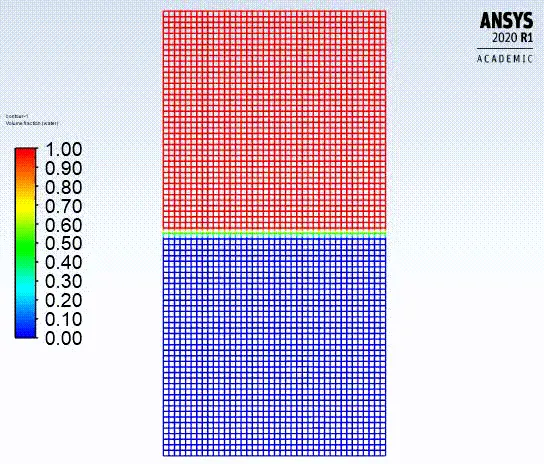
A baseline mesh for the given computational domain was created with default element size of 0.5mm, illustrated in Fig. 2. Since, the domain does not have any complex features, the default mesh created contains quad cells predominantly, which is of the highest quality in a two-dimensional computational domain, thereby keeping the cell count low, improving the computational time and reducing errors in solution calculation due to numerical diffusion.

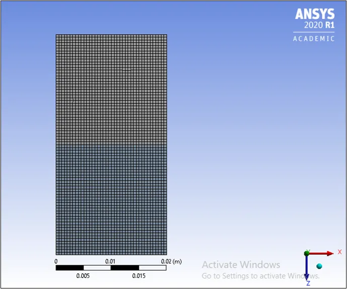
Fig. 2: Baseline Mesh

Mesh statistics and volume fraction for water values for Baseline Mesh:

Mesh	Element-Size(m)	Nodes	Elements	volume fraction for water
Baseline	5e-04	3321	3200	0.497

Table 2: Mesh statistics and volume fraction for water values for Baseline Mesh

Mesh quality attributes for Baseline Mesh:

Mesh	Element Quality(avg.)	Aspect Ratio(avg.)	Skewness(avg.)	Orthogonal Quality(avg.)
Baseline	0.99934	Quadrilaterals-1.0002	1.906e-004	1.0

Table 3: Mesh quality attributes depicting the average values of element quality, aspect ratio, skewness and orthogonal quality for Baseline mesh

From the statistics and the quality attributes of the Baseline mesh in Table 2 and Table 3 respectively, it can be ascertained that the mesh quality lies in the range of 'very good' to 'excellent' scale for the element size of 0.5mm with an almost perfectly stable predicted value of volume fraction for water at 0.497.

Section 2.4.2 Refined Mesh

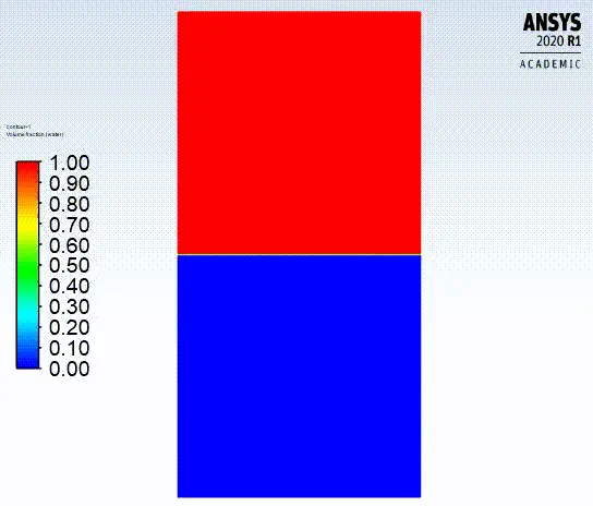
Similar to the Baseline Mesh, a refined mesh for the given computational domain was created with an element size of 0.1mm as seen in Fig. 3. The type of cells for the refined mesh were also quad dominant due to simplicity of the domain construction.

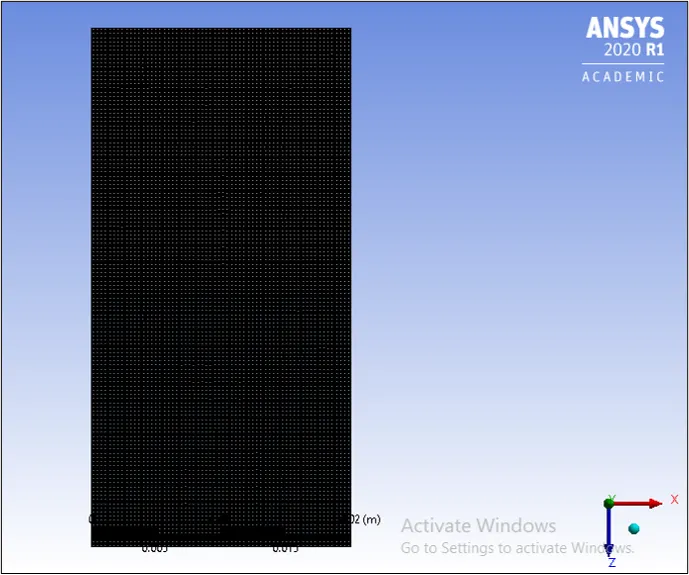
Fig. 3: Refined Mesh

Mesh statistics and volume fraction for water values for Refined Mesh:

Mesh	Element-Size(m)	Nodes	Elements	volume fraction for water - Air and Water as phases	volume fraction for water - user-defined material and Water as phases
Refined	1e-04	80601	80000	0.4904	0.4577

Table 4: Mesh statistics and volume fraction for water values for Refined Mesh

Mesh quality attributes for Refined Mesh:

Mesh	Element Quality(avg.)	Aspect Ratio(avg.)	Skewness(avg.)	Orthogonal Quality(avg.)
Refined	0.9988	Quadrilaterals-1.0007	8.8112e-004	0.99999

Table 5: Mesh quality attributes depicting the average values of element quality, aspect ratio, skewness and orthogonal quality for Refined mesh

The statistics and quality attributes of the Refined mesh in Table 4 and Table 5 respectively, just like the Baseline mesh, indicate that the mesh quality lies in the range of 'very good' to 'excellent' scale for the element size of 0.1mm owing to the domain's simplicity in design construction. The volume fraction for water predicted with the Refined mesh that includes Air and Water as phases results in an almost stable value of 0.4904. The minimum percentage variation (%var) of the volume fraction for water values with Air and Water as phases between the Baseline mesh and Refined mesh is about 1.328% which is almost negligible considering the difference in the number of elements between the two meshes. The %var is calculated as the ratio of the difference, in this case, of the volume fraction for water values in two consecutive meshes to the volume fraction for water of the previous mesh for Air and Water as phases i.e., ((volume fraction for water for Refined mesh - volume fraction for water for Baseline mesh)/volume fraction for water for Baseline mesh).

2.4.3 Convergence Level

In the given numerical analysis, Pressure based solver of type SIMPLE scheme was utilised. SIMPLE scheme by definition is iterative in nature, robust (memory efficient) and is quicker per iteration than other pressure-based solvers. The selection of schemes for the different terms under spatial discretization includes assigning Gradient to Least Squares Cell Based scheme, Pressure to PRESTO! scheme, Momentum to second order upwind scheme and Volume Fraction to Compressive scheme. For Transient Formulation, the scheme was set to First Order Implicit. Least Squares Cell Based scheme is the default gradient method chosen by ANSYS Fluent which is used to compute the change in values across the centroid of two cells along a vector path and is a computationally less expensive scheme offering comparable accuracy to the node-based gradient scheme, both of which are superior to the cell-based gradient scheme. PRESTO! scheme, which stands for PREssure STaggering Option, is the default scheme for pressure spatial discretization when the VOF Multiphase model is enabled and it makes use of a discrete continuity balance for a "Staggered" control volume about the face to compute the required pressure on it and is generally considered to indicate physically accurate results as it avoids interpolations and the associated errors due to it. A second order upwind scheme is chosen for the momentum spatial discretization that makes use of the quantities at the cell face values to compute a cell-centered solution at the cell centroid leading to a second order accurate solution. Compressive scheme for the Volume Fraction spatial discretization uses a second order reconstruction scheme which is evaluated based on the value of the slope limiter and is dependent on the type of interface regime modelling selected for a numerical analysis. Slope limiters prevents the occurrence of spurious oscillations or wiggles that are otherwise bound to be generated when using spatial discretizations of higher order. Compressive scheme is also applicable for the given analysis as the meshes generated are of good quality and yields better accuracy when compared against Modified HRIC in most cases as these two schemes are the only options available based on the configuration selected. The selection of First Order Implicit scheme for Transient Formulation was done primarily to observe the RTI phenomena using large time-step sizes despite it tending to produce more numerical diffusion when compared to either the Second Order Implicit or Bounded Second Order Implicit schemes as a result of limitations in computational resources mentioned previously. Convergence criteria option was retained and the residual values which measures the local imbalance of conserved variable in each control volume such as continuity, x-velocity, y-velocity, and vf-water were monitored throughout the solution process for the defined number of time steps to allow the actual fluid behaviour to be developed i.e., the formation of structures like spikes, bubbles, mushrooms, etc., as part of the different stages of the RTI phenomena, before the phases begin to settle in the domain based on their corresponding density values. The residual limits defined for the laminar viscous model and VOF Multiphase model equations and the residual plots corresponding to the different meshes are shown in the table and figures below:

	laminar	VOF Multiphase
continuity	1e-03	--
x-velocity	1e-03	--
y-velocity	1e-03	--
vf-water	--	1e-03

Table 6: Residual Values of the different equations used in the laminar and VOF Multiphase model

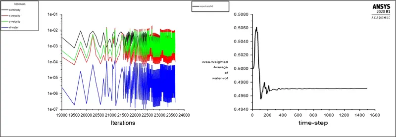
Fig. 4: Scaled Residuals and volume fraction for water plots using laminar viscous model in transient state with Water and Air as phases for Baseline mesh with SIMPLE solver

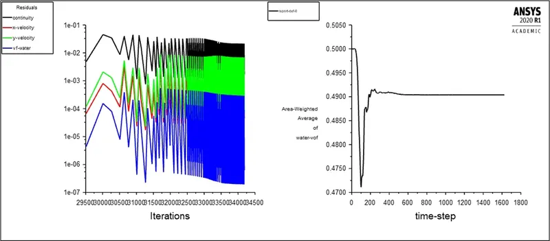
Fig. 5: Scaled Residuals and volume fraction for water plots using laminar viscous model in transient state with Water and Air as phases for Refined mesh with SIMPLE solver

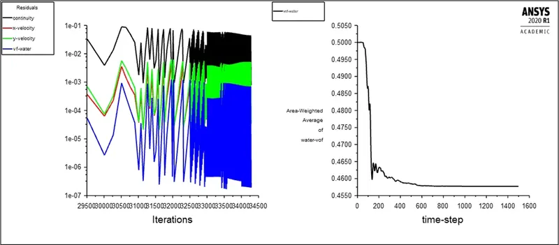
Fig. 6: Scaled Residuals and volume fraction for water plots using laminar viscous model in transient state with user-defined material and Water as phases for Refined mesh with SIMPLE solver

From Fig. 4, Fig. 5 and Fig. 6, we can notice that while the residuals show a particular trend in calculation of values which remains consistent throughout the solution process as they progress towards convergence through different time steps, it is only for about the initial time-step range from 0 to 600 in the area-weighted average of volume fraction for water value estimation that fluctuations are observed which is synonymous with the interactions that occur between the phase materials of the given domain giving rise to the formation of structures like spikes, bubbles, mushrooms, etc., before the flow begins to stabilise. It is important to note that while the Baseline Mesh with Air and Water as phase materials and Refined Mesh with user-defined material and Water as phase materials make use of a larger time-step size of 0.005s for 1500 number of time-steps with maximum iterations per time step to 25, the same was not possible to be achieved for the Refined Mesh with Air and Water as phase materials as it resulted in an error of floating point exception. This was because the velocity of flow in the domain during the initial iterations are still low resulting in the corresponding value of Courant Friedrichs Lewy (CFL) condition to be large which eventually causes the residuals to change by a drastically high value. Therefore, the simulations for Refined Mesh with Air and Water as phase materials was carried out with a time-step size of 0.001s set at 3000 number of time-steps with maximum iterations per time step to 25, although after 1600 iterations the monitor report did not show any fluctuations in values with an almost steady output of volume fraction for water predicted as was the solution reaching convergence per time step in fewer iterations.

3.Results and Discussion

In Section 3.1, numerical simulation results for the RTI phenomena and volume fraction for water are compared between the Baseline Mesh and the Refined Mesh for Water and Air as phase materials as well as compared against user-defined material and Water for the latter mesh.

3.1. Numerical results for RTI phenomena and volume fraction for water

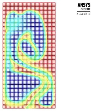
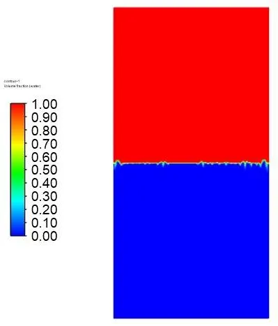
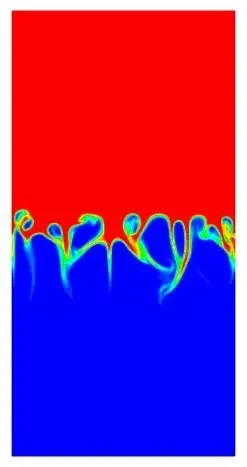
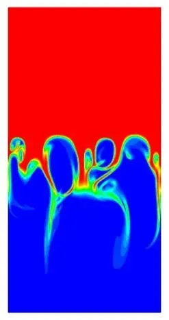
The growth of RTI phenomena takes place through different stages. The first stage is described by the presence of initial perturbations of extremely small velocity field or amplitudes which are smaller when compared to their wavelengths and as such can be analysed using linearised form of dynamical equations for the fluid leading to the exponential instability growth (seen in Fig. 8 a), 9 a) and 10 a) respectively). The second stage is typically observed after the perturbations grow non-linearly to a wavelength size of order `lambda` and its development is governed by the presence of three dimensional effects and Atwood number. Atwood number dictates the penetration distance of heavy fluid bubbles into the lighter fluid bubbles thereby also indicating the time taken for the subsequent Rayleigh-Taylor mixing and is expressed mathematically as function of acceleration time scale i.e., `A*g*t^2`. For Air and Water as phases, the Atwood number based on its definition, as mentioned in Section 1. Introduction, results in a value of 0.9975 while for user-defined material and Water as phases the value yielded is 0.4278. In the case of Air and Water phase materials, since the resulting Atwood number corresponds to a value close to 1, it implies that the movement of light fluid into the heavy fluid is in the form of round topped bubbles with circular cross sections as can be seen in Fig. 8 b) and Fig. 9 b), while in the case of user-defined material and Water as phase materials the bubbles from both materials tend to be more interpenetrating as seen in Fig. 10 b) and this resonates well with the influence of Atwood number stated before for the RTI phenomena. In the third stage, spikes begin to appear between different bubbles as well as the bubbles begin to interact amongst themselves. Initial perturbations interact non-linearly among each other and at frequencies inconsistent across the deforming interface. In case of lower density ratios such as the one observed with user-defined material and Water as phase materials in Fig. 10 c), Helmholtz instability, another type of hydrodynamic instability, takes place due to discontinuity in the velocity and density profiles at the interface thereby inducing vorticity that appears as an unstable vortex sheet rolling into a spiral which promotes the growth of mushroom shaped structures along the sides of the spike causing increase in drag force effects on the same. For lower density ratios than that observed with user-defined material and Water as phase materials, the process of bubble amalgamation indicated by the absorption of small bubbles by larger bubbles is also evident as was confirmed through experimental findings. The fourth stage, which also resembles the last stage in the development of the RTI phenomena, is observed by the collapse of the spike which takes place through different mechanisms. It is in this stage where turbulent mixing takes place (seen in Fig. 8 d), 9 d) and 10 d) respectively), although dependent on the Reynolds number to be large. Between the Baseline Mesh and the Refined mesh for Air and Water as phase materials in the domain, we can clearly notice that the interface thickness to be smaller on the refined mesh in Fig. 9 a) in comparison to Fig. 8 a) of the Baseline Mesh. Similarly, Fig. 9 b) and Fig. 9 c) of the Refined Mesh represent the formation of different bubble sizes more clearly and the region of spikes generation along with interaction amongst bubbles appears with a much more sharper resolution respectively than that of the Baseline Mesh in Fig. 8 b) and Fig. 8 c). This can be attributed to the fact that the numerical diffusion has significantly reduced as a result of mesh refinement in addition to the implementation of a smaller time-step size, as was accounted for before due to an error of floating point exception.

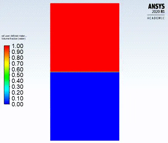a) Air, Water (phase materials) - Baseline Mesh b) Air, Water (phase materials) - Refined Mesh c) UD, Water (phase materials) - Refined Mesh

Fig. 7: Stages of development in RTI phenomena across different phase materials and meshes (UD: user-defined)

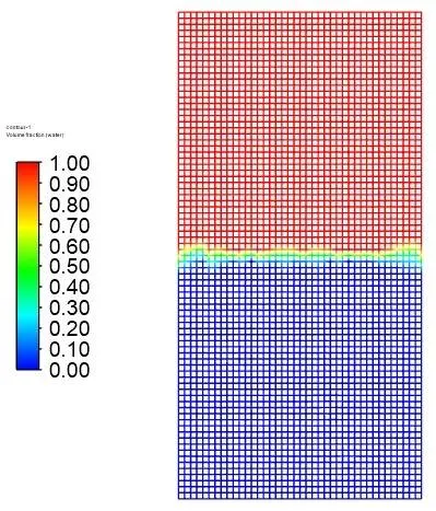
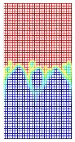
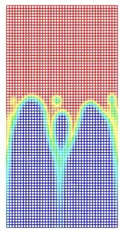
a) Stage 1 - Initial perturbations b) Stage 2 - Bubble formations c) Stage 3 - Spikes between bubbles d) Onset of turbulent mixing

Fig. 8: Stages of development in RTI phenomena with Air and Water as phase materials for Baseline Mesh

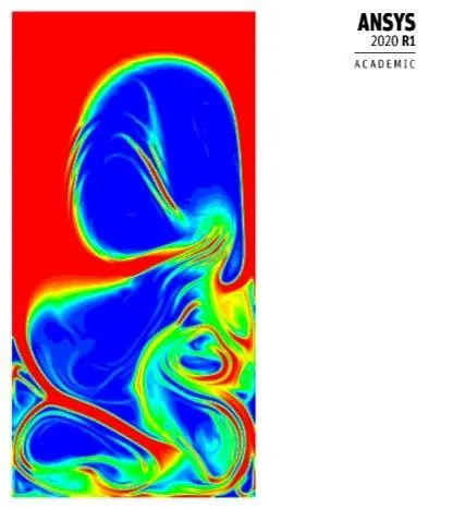
a) Stage 1 - Initial perturbations b) Stage 2 - Bubble formations c) Stage 3 - Spikes between bubbles d) Onset of turbulent mixing

Fig. 9: Stages of development in RTI phenomena with Air and Water as phase materials for Refined Mesh

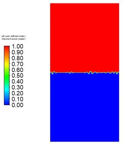
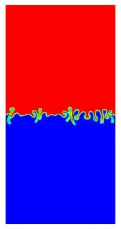
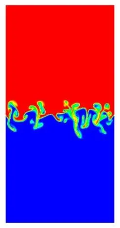
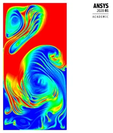
a) Stage 1 - Initial perturbations b) Stage 2 - Interpenetrating bubbles c) Stage 3 - Mushroom structures d) Onset of turbulent mixing

Fig. 10: Stages of development in RTI phenomena with user-defined material and Water as phase materials for Refined Mesh

5. Conclusion

The numerical analysis for the RTI phenomena with Air and Water as phases in one domain and user-defined material and Water as phases in another domain under transient conditions using the laminar viscous and VOF Multiphase model in ANSYS Fluent 2020 R1 was well understood. It was realised that while the first stage of the RTI phenomena due to its relatively small velocity field or amplitudes smaller to its wavelengths could be computed using linear form of dynamical equations, the underlying influence of the density ratio or Atwood number governed the formation of different structures in the latter stages of fluid flow development which subsequently determined the interaction between them that would eventually deciding whether the regime of chaotic mixing would be arrived to earlier or later. The analysis of the RTI phenomena carried out in this numerical analysis does not consider the role of other real world scenarios such as surface tension, viscosity, etc., and that the accuracy of the obtained solution could improve with further reduction in the time-step size, however, the overall instability behaviour with the formation of structures like spikes, bubbles, mushrooms, etc., was well observed using the CFD model configured for the given setup across its different stages.

6. References

[1] D.L. Youngs, Numerical simulation of turbulent mixing by Rayleigh-Taylor instability, Physica D 12 (1984) 19.

[2] D.L. Youngs, Modelling Turbulent Mixing by Rayleigh-Taylor instability, Physica D 37 (1989) 270-287.