Week 5 - Curve fitting
1. Introduction
Curve fitting can be described as a process of modelling or representing a dataset by allocating a mathematical function that would be considered as a best fit across all the data points. Common types of curve fitting includes interpolation, which refers to a function that would exactly fit the given dataset, and smoothing, which points to a function that would be a more approximate fit to the same dataset in the light of similar comparison. The former technique finds limited use from the perspective of real-life scenarios while the latter finds more applications to relate to but does lead to errors which needs to be ensured that they are minimised for a better characterisation. In most cases and with increasing importance of data analysis in different industries, curve fitting is seen as a valuable data visualisation aid for capturing trends and forecasting future possible events, and in some situations to deduce values from a function with no historical data as well as obtain relationships between different variables. The aim of this programming exercise was to perform curve fitting on a given Cp vs Temperature data file and evaluate goodness of fit and error criteria across different types of functions.
2. Method
2.1 Modelling
The problem was solved by building a mathematical model in Python using the Sublime Text source code editor (code snippet for which is attached with this report) along with the math and numpy modules/libraries for defining mathematical expressions, and creating arrays and its corresponding expressions respectively. Additionally, and to perform curve fitting, the curve fit function from the scipy.optimize package is used. Scipy is a scientific computing module of Python that provides a number of in-built functions developed for many well-known mathematical functions with curve fit being one of them that makes use of non-linear least squares to fit a given or desired function to data. Similarly, the mean function is accessed to perform arithmetic mean from the statistics module which contains other similar functions for evaluating mathematical statistics of a given dataset.
2.2 Mathematical Model Setup
A curve fit function in Python is syntaxed as shown below:
`text(scipy.optimize.curve_fit(f, xdata, ydata[, p0, sigma, …]))`; where (1)
`f` is the function, in this case `f(text(temperature))`,
`text(xdata)` is the independent variable for which data is measured, in this case temperature,
`text(ydata)` is the dependent data, in this case Cp, and
`[, p0, sigma, …]` are additional arguments of which `p0` and `text(sigma)` being initial guess for parameters and determination of uncertainty in `text(ydata)` respectively
The values returned from the curve fit function in Eq. (1) are popt and pcov which are an array and 2D array respectively. popt represents the optimal values for the parameters such that the sum of the squared residuals of `f(text(xdata, *popt)) - text(ydata))` is minimized. pcov refers to the estimated covariance of popt wherein the diagonals of the 2D array gives the variance of the parameter estimate [1]. Since, the popt argument consists of the best-fit values of the coefficients describing the function which are generally more than one, the '*' before popt indicates that all of these values are required to be selected or considered, and this comes in handy especially when the polynomial function contains many terms involving multiple coefficients. In the given problem, a fit for the linear and cubic polynomial functions were created for the Cp data as shown below:
Linear function:
`text(func_linear) = a*t + b`; where (2)
`a` and `b` are the coefficients, and
`t` is the temperature
Cubic polynomial function:
`text(func_cubic_polynomial) = a*t^3 + b*t^2 + c*t + d`; where (3)
`a`, `b`, `c` and `d` are the coefficients
Values of temperature that are to be utilised by the linear and cubic polynomial function are passed as a NumPy array using the function np.array() with temperature as the argument to provide ease in handling of arithmetic operations because of a relatively straightforward and direct approach rather than if the same variable were to be of list type as was its initial declaration. In order to evaluate the goodness of fit and error criteria across different types of functions, it was decided to first create plot of residuals i.e., difference between actual data and fitted data, versus the fitted data for each curve fitting function to understand if the models were biased (fitted values are at extreme positions with regards to actual data) followed by determining the respective R-squared (`R^2`) quantities. R-square is a ratio of the amount of variance captured by the model to the amount of variance present in the model. Mathematically, R-square equates to the ratio of sum of squares of regression to the total sum of squares with the formulations of each term further highlighted below:
`R^2 = (SSR)/(SST)`; where (4)
`SSR` is the sum of squares of differences between the values of the fitting function at their respective points and the arithmetic mean of the dataset equating to `sum_(i=0)^n(f(x(i))-text(mean))^2`,
`SST` is the sum of squares of regression, `SSR`, and sum of squares of errors, `SSE`, wherein `SSE = sum_(i=0)^n|y(i)-f(x(i))|^2` with `y(i)` representing the actual data point
Typically, closer the value of R-square to 1, better is the fit. In order to make the curve fit perfect, it was decided to adopt either the linear or cubic polynomial function, based on the minimum of the two in terms of the overall sum of residuals, and perform a split-wise approach of the resulting curve fit by giving the option to choose a value for number of splits that is both positive and even.
3. Results
3.1 Curve fitting using linear, cubic polynomial functions and evaluation of goodness of fit and error criteria including residuals
Fig.1 and Fig. 2 below captioned 'Plot of comparison of residual values vs fitted values for different curve fit functions' and 'Plot of comparison of different curve fit functions on Cp vs Temperature data' shows the values computed for residuals and Cp respectively for different curve fit functions. It can be observed that the residuals for linear curve fit are significantly larger and this decreases for the cubic polynomial and its split-wise approach function with eight splits. Additionally, and because of decreasing trend in residuals values, it can be noticed that for a higher degree polynomial function and even more so for the same function implemented using a split-wise approach, it appears to be visually a better fit which is also assured from the R-square values, an indication of goodness-of-fit measure. It should be noted that the residual values shown in Fig. 1 have points skipped at intervals of 100 for enhanced visualisation without comprising on the actual trend or behaviour.
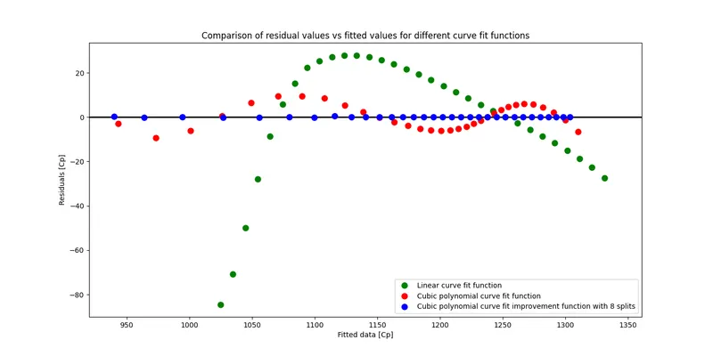
Fig. 1: Plot of comparison of residual values vs fitted values for different curve fit functions
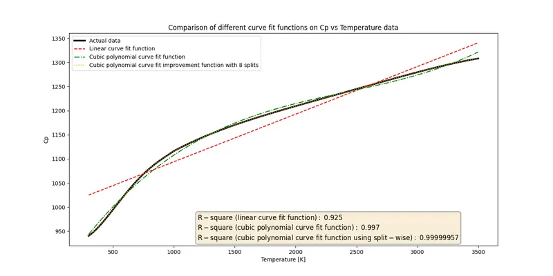
Fig. 2: Plot of comparison of different curve fit functions on Cp vs Temperature data
4. Discussion
The evaluation of residual values for different curve fit functions reveals that with respect to the actual or observed data, positive values means predictions were low, negative values means predictions were high while zero means that it was a perfect match. Moreover, the linear function exhibits residuals that are in general far away from the ideal value of zero while in the case of the cubic polynomial function (without the split-wise approach) demonstrates a trend of curving up and down with almost similar peak amplitudes and a recognisable pattern, almost like a sine function. Both these functions, based on the residual plots, indicates that the consequent models are biased with the former function more so as density of points close to the origin are low but away from the origin are high apart from the consistent under and over-prediction of the data along the curve making the results not entirely reliable. This behaviour is however diminished or almost non-existent when the split-wise approach is chosen for the cubic polynomial function, which was found to have the lowest sum of overall residuals, and the value of R-square for the same also indicating the best fit out of the given functions.
5. Conclusion
The determination of different curve fit functions, and evaluation of their residual and R-square values to estimate goodness of fit in Python using the Sublime Text source code editor was well understood with this programming exercise. It was realised that understanding the model's behaviour in terms of being biased or not is foremost necessary as high R-square value does not guarantee if a regression model would prove to be an adequate fit to a given dataset with this being one of the major limitations of R-square as a goodness of fit measure and that an unbiased residual plot also provides key insights in terms of the relationship between different variables. The applications of curve fitting have now grown many folds with rapid expansion across different industries, including in engineering applications, and the importance of the same is helping companies to aim for improved productivity and lower operational costs while also achieving rise in profits.
References
[1] SciPy documentation, scipy.optimize.curve_fit, https://docs.scipy.org/doc/scipy/index.html, viewed 10 December 2021, <https://docs.scipy.org/doc/scipy/reference/generated/scipy.optimize.curve_fit.html#scipy.optimize.curve_fit>
CODE:
Program to perform curve fitting on Cp vs Temperature data file and evaluate goodness of fit and error criteria including plotting of residuals.
# Program to perform curve fitting on Cp vs Temperature data file and evaluate goodness of fit and error criteria including plotting of residuals.
# Author: Diptesh Pawa

# Modules/Libraries
import math
import matplotlib.pyplot as plt
import numpy as np
from scipy.optimize import curve_fit
from statistics import mean

# Initialisation
# Sum of squares due to error (SSE) and Sum of squares due to regression (SSR) terms for the concerned curve fit functions
SSE_actual_linear = 0
SSE_actual_cubic_polynomial = 0
SSR_actual_linear = 0
SSR_actual_cubic_polynomial = 0
residual_actual_linear = []
residual_actual_linear_splitwise = []
residual_actual_cubic_polynomial = []
residual_actual_cubic_polynomial_splitwise = []

# Curve fit functions
def func_linear(t, a, b):
	return a*t + b

def func_cubic_polynomial(t, a, b, c, d):
	return a*pow(t,3) + b*pow(t,2) + c*t + d

# Reading thermodynamic data file
def read_file():
	temperature = []
	cp = []
	for line in open('data','r'):
		values = line.split(',')
		temperature.append(float(values[0]))
		cp.append(float(values[1]))

	return [temperature,cp]

# Main Program
temperature,cp = read_file()

# Curve fit using linear and cubic polynomial equations for the Cp data
popt_linear, pcov_linear = curve_fit(func_linear, temperature, cp)
popt_cubic_polynomial, pcov_cubic_polynomial = curve_fit(func_cubic_polynomial, temperature, cp)
fit_cp_linear = func_linear(np.array(temperature), *popt_linear)
fit_cp_cubic_polynomial = func_cubic_polynomial(np.array(temperature), *popt_cubic_polynomial)

# Evaluation of best curve fit by determining R-square quantities
mean_cp_linear = mean(fit_cp_linear)
mean_cp_cubic_polynomial = mean(fit_cp_cubic_polynomial)

for i in range(0,len(cp)):
	residual_actual_linear = np.append(residual_actual_linear,cp[i] - fit_cp_linear[i])
	residual_actual_cubic_polynomial = np.append(residual_actual_cubic_polynomial,cp[i] - fit_cp_cubic_polynomial[i])
	SSE_actual_linear = SSE_actual_linear + pow(cp[i] - fit_cp_linear[i], 2)
	SSE_actual_cubic_polynomial = SSE_actual_cubic_polynomial + pow(cp[i] - fit_cp_cubic_polynomial[i], 2)
	SSR_actual_linear = SSR_actual_linear + pow(fit_cp_linear[i] - mean_cp_linear, 2)
	SSR_actual_cubic_polynomial = SSR_actual_cubic_polynomial + pow(fit_cp_cubic_polynomial[i] - mean_cp_cubic_polynomial, 2)

#print('residual_actual_linear = ', residual_actual_linear)
SST_actual_linear = SSE_actual_linear + SSR_actual_linear
SST_actual_cubic_polynomial = SSE_actual_cubic_polynomial + SSR_actual_cubic_polynomial
R_square_actual_linear = SSR_actual_linear/SST_actual_linear
R_square_actual_cubic_polynomial = SSR_actual_cubic_polynomial/SST_actual_cubic_polynomial

# Curve fit improvement using the split-wise approach
fit_cp_linear_splitwise = []
fit_cp_cubic_polynomial_splitwise = []

# Sum of squares due to error (SSE) and Sum of squares due to regression (SSR) terms for the concerned curve fit improvement functions
SSE_actual_linear_splitwise = 0
SSE_actual_cubic_polynomial_splitwise = 0
SSR_actual_linear_splitwise = 0
SSR_actual_cubic_polynomial_splitwise = 0

x = y = 0
splits_input_invalid_entry = 'Y'

# Condition to check for entry regarding number of splits as an even number
splits = int(input('Please enter an even number for splits or ranges to perform curve fit improvement using the split-wise approach: '))
while splits_input_invalid_entry == 'Y':
	if (splits % 2) == 0 and splits != 0 and splits > 0 and splits <= len(cp):
		splits_input_invalid_entry = 'N'
	else:
		splits = int(input('The number entered is either not an even number or zero or negative or exceeds the length of cp range. Kindly re-enter a positive even number: '))

# Curve fit improvement functions using either linear or cubic polynomial equations for the Cp data as well as evaluation of goodness of fit and error criteria by determining R-square quantities
if sum(residual_actual_cubic_polynomial)<sum(residual_actual_linear):
	for i in range(0,splits):
		y = int((x + (len(cp)/splits)))
		popt_cubic_polynomial_splitise, pcov_cubic_polynomial_splitise = curve_fit(func_cubic_polynomial, temperature[x:y], cp[x:y])
		fit_cp_cubic_polynomial_splitwise = np.append(fit_cp_cubic_polynomial_splitwise,func_cubic_polynomial(np.array(temperature[x:y]), *popt_cubic_polynomial_splitise))
		x = int(y)
	mean_cp_cubic_polynomial_splitwise = mean(fit_cp_cubic_polynomial_splitwise)
	for i in range(0,len(cp)):
		residual_actual_cubic_polynomial_splitwise = np.append(residual_actual_cubic_polynomial_splitwise,cp[i] - fit_cp_cubic_polynomial_splitwise[i])
		SSE_actual_cubic_polynomial_splitwise = SSE_actual_cubic_polynomial_splitwise + pow(cp[i] - fit_cp_cubic_polynomial_splitwise[i], 2)
		SSR_actual_cubic_polynomial_splitwise = SSR_actual_cubic_polynomial_splitwise + pow(fit_cp_cubic_polynomial_splitwise[i] - mean_cp_cubic_polynomial_splitwise, 2)
	SST_actual_cubic_polynomial_splitwise = SSE_actual_cubic_polynomial_splitwise + SSR_actual_cubic_polynomial_splitwise
	R_square_actual_cubic_polynomial_splitwise = SSR_actual_cubic_polynomial_splitwise/SST_actual_cubic_polynomial_splitwise
	textstr = '\n'.join((
	r'$\mathrm{R-square \ (linear \ curve \ fit \ function): \ }%.3f$' % (R_square_actual_linear,),
	r'$\mathrm{R-square \ (cubic \ polynomial \ curve \ fit \ function): \ }%.3f$' % (R_square_actual_cubic_polynomial, ),
	r'$\mathrm{R-square \ (cubic \ polynomial \ curve \ fit \ function \ using \ split-wise): \ }%.8f$' % (R_square_actual_cubic_polynomial_splitwise, )))
else:
	for i in range(0,splits):
		y = int((x + (len(cp)/splits)))
		popt_linear_splitise, pcov_linear_splitise = curve_fit(func_linear, temperature[x:y], cp[x:y])
		fit_cp_linear_splitwise = np.append(fit_cp_linear_splitwise,func_linear(np.array(temperature[x:y]), *popt_linear_splitise))
		x = int(y)
	mean_cp_linear_splitwise = mean(fit_cp_linear_splitwise)
	for i in range(0,len(cp)):
		residual_actual_linear_splitwise = np.append(residual_actual_linear_splitwise,cp[i] - fit_cp_linear_splitwise[i])
		SSE_actual_linear_splitwise = SSE_actual_linear_splitwise + pow(cp[i] - fit_cp_linear_splitwise[i], 2)
		SSR_actual_linear_splitwise = SSR_actual_linear_splitwise + pow(fit_cp_linear_splitwise[i] - mean_cp_linear_splitwise, 2)
	SST_actual_linear_splitwise = SSE_actual_linear_splitwise + SSR_actual_linear_splitwise
	R_square_actual_linear_splitwise = SSR_actual_linear_splitwise/SST_actual_linear_splitwise
	textstr = '\n'.join((
	r'$\mathrm{R-square \ (linear \ curve \ fit \ function): \ }%.3f$' % (R_square_actual_linear,),
	r'$\mathrm{R-square \ (cubic \ polynomial \ curve \ fit \ function): \ }%.3f$' % (R_square_actual_cubic_polynomial, ),
	r'$\mathrm{R-square \ (linear \ curve \ fit \ function \ using \ split-wise): \ }%.8f$' % (R_square_actual_linear_splitwise, )))

# Plotting of residuals for different curve fit functions highlighting their relative errors in prediction and understanding bias in them, if any
fig, ax = plt.subplots(figsize=(14, 7))
ax.axhline(y = 0, color = 'k', linestyle = '-', linewidth=2)
linear_curve_fit_residuals, = ax.plot(fit_cp_linear,residual_actual_linear, color='green', linestyle='None', marker='o', markersize=8, markevery=100, label = 'Linear curve fit function')
cubic_curve_fit_residuals, = ax.plot(fit_cp_cubic_polynomial,residual_actual_cubic_polynomial, color='red', linestyle='None', marker='o', markersize=8, markevery=100, label = 'Cubic polynomial curve fit function')
if len(residual_actual_cubic_polynomial_splitwise) != 0:
	cubic_curve_fit_improvement_residuals, = ax.plot(fit_cp_cubic_polynomial_splitwise,residual_actual_cubic_polynomial_splitwise, color='blue', linestyle='None', marker='o', markersize=8, markevery=100, label = "Cubic polynomial curve fit improvement function with {} splits".format(splits))
	plt.legend(handles=[linear_curve_fit_residuals, cubic_curve_fit_residuals, cubic_curve_fit_improvement_residuals])
else:
	linear_curve_fit_improvement_residuals, = ax.plot(fit_cp_linear_splitwise, residual_actual_linear_splitwise, color='blue', linestyle='None', marker='o', markersize=8, markevery=100, label = "Linear curve fit improvement function with {} splits".format(splits))
	plt.legend(handles=[linear_curve_fit_residuals, cubic_curve_fit_residuals, linear_curve_fit_improvement_residuals])
plt.ylabel('Residuals [Cp]')
plt.xlabel('Fitted data [Cp]')
plt.title('Comparison of residual values vs fitted values for different curve fit functions')
plt.savefig('Week_5_residuals_vs_fitted_data.png')

# Plotting of actual data, curve fit functions and their associated goodness of fit through R-square quantities
fig_2, ax_2 = plt.subplots(figsize=(14, 7))
props = dict(boxstyle='round', facecolor='wheat', alpha=0.5)
ax_2.text(0.3, 0.15, textstr, transform=ax.transAxes, fontsize=12, verticalalignment='top', horizontalalignment='left', bbox=props)
data, = ax_2.plot(temperature, cp, label = 'Actual data', color = "black", linewidth = 3)
linear_curve_fit_function, = ax_2.plot(temperature, fit_cp_linear, label = 'Linear curve fit function', color = "red", linewidth = 1.5, linestyle='--')
cubic_curve_fit_function, = ax_2.plot(temperature, fit_cp_cubic_polynomial, label = 'Cubic polynomial curve fit function', color = "green", linewidth = 1.5, linestyle='-.')
if sum(residual_actual_cubic_polynomial)<sum(residual_actual_linear):
	cubic_curve_fit_improvement_function, = ax_2.plot(temperature, fit_cp_cubic_polynomial_splitwise, label = "Cubic polynomial curve fit improvement function with {} splits".format(splits), color = "orange", linewidth = 1.5, linestyle = 'dotted')
	plt.legend(handles=[data, linear_curve_fit_function, cubic_curve_fit_function, cubic_curve_fit_improvement_function])
else:
	linear_curve_fit_improvement_function, = ax_2.plot(temperature, fit_cp_linear_splitwise, label = "Linear curve fit improvement function with {} splits".format(splits), color = "orange", linewidth = 1.5, linestyle = 'dotted')
	plt.legend(handles=[data, linear_curve_fit_function, cubic_curve_fit_function, linear_curve_fit_improvement_function])
plt.xlabel('Temperature [K]')
plt.ylabel('Cp')
plt.title('Comparison of different curve fit functions on Cp vs Temperature data')
plt.savefig('Week_5_curve_fitting_C_p_vs_T.png')

plt.show()