Week 7: Shock tube simulation project

1. Introduction

A shock tube can be described as a device, generally used in a laboratory setup, that produces high-temperature, high-pressure gases whose thermodynamic and chemical properties are subsequently assessed. The typical construction of a shock tube involves a very long pipe, closed at either ends, and consisting of a diaphragm that separates the high and low pressure regions, also known as the "Driver" and "Driven" sections respectively, within which a considerably strong shock wave can be created and transmitted. More importantly, gases in either regions can be at different temperatures and have different molecular weights making shock tubes greatly advantageous in applications such as testing of supersonic bodies and hypersonic entry vehicles and finding even more prominence towards development of high-power gasdynamic and chemical lasers.

The aim of this challenge was to perform three-dimensional, transient state simulations using the default physical model without turbulence modelling to solve the compressible form of Navier-Stokes equations for a shock tube configuration in which the breaking of the diaphragm was controlled by the time set in the "Events" feature of CONVERGE and then computing the flow properties across the domain. The analysis involved verification and validation of the computational model using gases of same molecular weights, in this case air, and at same temperatures in the high and low pressure regions in order to facilitate easier comparison against the analytical solutions for pressure, density, temperature and velocity across the domain, whose formulations are reported by John D. Anderson, Jr. in [1], as well as stating the total cell count and mesh quality attributes like skewness, non-orthogonality and aspect ratio in all cases.

2. Method

The typical approach adopted to performing numerical simulations in CONVERGE CFD involves the following steps:

1. Creating a new folder dedicated to running the concerned project inside a user-preferred directory.
2. Setting up the relevant case file(s) in Converge Studio v3.0 that involves creation of the fluid volume domain, setting up the required application type, choosing material and its state (in this case gas) for which simulation is to be performed along with the requisite properties, defining simulation parameters such as solver types, run time variables, and convergence tolerances, defining regions, boundary conditions and initial conditions, specifying the physical models whose equations are intended to be solved, allocating the base grid size values, and lastly selecting the variables for post-processing at the required time intervals along with any hidden parameters or UDF selection as part of advanced parameters.
3. Saving the case file(s) and exporting the input files into the folder created for running the concerned project which typically includes 'boundary.in' for the various boundary conditions, 'material_state.dat' where material_state points to 'gas' in this case, 'initialize.in' specifying initial conditions, 'inputs.in' defining the various input conditions and file writing intervals, 'post.in' for the different post-processing variables, 'solver.in' describing the solver chosen and its equations, and 'surface.dat' containing datasets about the surface while other input files with respect to the state of the material, thermal properties and species may also be part of the exporting process and should be ensured that they are selected for the simulation to run.
4. Running the simulation in a Cygwin64 terminal window.
5. Post-converting 3D output data by navigating to the output folder created within the same project folder during the simulation run or from the 'Post-Processing 3D' button in Converge Studio v3.0.

The simulation run and post-converting processes were executed using Linux-type commands in a Cygwin64 terminal window as shown below:

i) Change directory to the project containing the relevant case file(s):

cd "PATH_TO_CONCERNED_PROJECT_FOLDER"

ii) Confirm the contents of the project for the exported input files:

ls

iii) Performing simulation run with the converge executable application on multiple processors (in this case, 4) using mpiexec executable file in the background (by adding ampersand operator) along with posting output into a logfile:

mpiexec.exe -n 4 converge.exe restricted </dev/null> logfile &

iv) Checking for simulation status with regards to completion or errors:

tail logfile

v) Post-converting the 3D output data files using the 'post_convert_30_msmpi_64' utility on multiple processors (in this case, 4) using mpiexec executable file from within the output folder of the project containing the exported input files:

cd output

mpiexec.exe -n 4 post_convert_30_msmpi_64

2.1 Modelling

The computational domain for performing transient simulation of air flow movement across the shock tube consisting of two different pressure regions partitioned by a diaphragm was modelled in Converge Studio v3.0. The length of the domain was chosen to be a value such that after the diaphragm was broken and a sufficient time was elapsed, the development of unsteady wave motion and its corresponding flow properties could be measured leading to the selection of 10m along the x-axis direction of the global coordinate system with the diaphragm located at the mid-position of 5m with respect to the same orientation and the height and width, aligned along the y-axis and z axis directions respectively, to be 1m each. The basic element entity in CONVERGE is denoted by a triangle which would be visible by clicking on any of the surfaces of the recently drawn model and in order to demarcate boundaries, the corresponding triangles need to be grouped together. The process of grouping and creating new boundaries began with clicking on the 'Boundary' button under the 'Geometry' dock which was followed by clicking on the '+' symbol from which the pop-out message would read as 'Create a new boundary.' leading to the 'Boundary definition' window to open in which the option 'Create multiple boundaries' was checked with the number of boundaries set to 2, in this case, followed by lastly grouping the triangles that constitute a given surface and naming them accordingly, such as 'HighPressureSlipWalls' and 'LowPressureSlipWalls' illustrated in Fig. 1. It should be especially noted that the diaphragm was not physically modelled by defining boundaries for the same but using the "Events" feature of CONVERGE that would control the timing and specification of concerned regions between which fluid flow would occur and therefore, any triangles present at the concerned location of the diaphragm were required to be deleted. Moreover, the normal from each of the triangular surface is required to point towards the fluid domain which was ensured by first visualising the same using the 'Normal toggle' button accessible in the 'View Toolbar' and depending on the direction along which the normal is pointing, a decision was taken by clicking on the 'Normal' tab within the 'Transform' button under the 'Geometry' dock and selecting the suitable option from one of the three 'Transform Normal Options' followed by clicking on the 'Apply' button. At this stage and for the given numerical analysis, the modelling requirements were achieved, however, to validate if the model was clean i.e., it contains no intersecting edges, overlapping triangles or any other form of geometrical constraints, a check was performed by clicking on the 'Find' button in the 'Diagnosis' dock to observe for any anomalous 'Problem Triangles' and rectify the same.

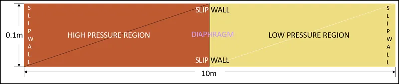
Fig. 1: Fluid Volume Model with the Diaphragm located at the center of the domain, Boundary Conditions and the 'High Pressure' and 'Low Pressure' regions in two-dimensional space

2.2 Meshing

The meshing approach adopted for the given computational domain was developed to maintain the meshing quality attributes viz., aspect ratio, skewness, and non-orthogonality as outlined in the CONVERGE 3.0 Manual [2] provided in the following table:

Aspect Ratio		1 (Ideal Value)
Skewness	0° (Ideal Value)	< 70° (Acceptable)	`>=` 90° (Likely to cause simulation failure)
Non-Orthogonality	0° (Ideal Value)	< 70° (Acceptable)	`>=` 90° (Likely to cause simulation failure)

Table 1: Mesh Quality Attributes as defined in the CONVERGE 3.0 Manual [2]

The reason for pursuing the above mentioned mesh quality attributes, as specified in Table 1, can be ascertained on the fact that whether the discretized domain was likely to create convergence issues during the solution process and also to identify areas in the mesh where the statistics can be improved based on the underlying physics. In Section 2.3.4 Mesh Refinement approach and selection of transient parameters for the given numerical simulation, detailed discussion about the different meshes that were prepared and their mesh qualities has been highlighted.

2.3 CFD Simulation Setup, Boundary Conditions and Monitoring Variables

The simulations on all meshes was performed using the default physical model consisting of no turbulence equations. A brief description into the working of the default physical model is provided below:

2.3.1 Default physical model

The default physical model can be described as the solution of the governing fluid equation viz., Navier-Stokes equations for a domain, in this case, discretized using the finite volume approach, without the presence of turbulence terms. The Navier-Stokes equations define the fluid flow properties such as velocity, pressure, density, temperature, viscosity, energy, etc., within a given physical domain. Additionally, the Navier-Stokes equations are developed with regards to the laws of conservation that states the net mass flow across a system is zero (Conservation of mass) and that the momentum within the same system (or control volume) is constant (Conservation of momentum). Since, energy is also a variable of assessment for the given numerical analysis, then according to the first law of thermodynamics, total heat gain of a system is equal to the sum of heat added to the system and work done on the same system.

2.3.1.1 Setup of the default physical model:

To use the default physical model in Converge Studio v3.0, we navigate to Physical Models option in the Case Setup tree and uncheck 'Turbulence modeling' to prevent inclusion of turbulence terms in the solution of governing flow equations.

2.3.2 Boundary Conditions and Monitoring Variables

The different boundary conditions for simulation of air flow movement across the two different pressure regions of the shock tube separated by a diaphragm is described in Table 2. Walls in both the high pressure and low pressure regions of the given domain were modelled as slip walls, a special case of the Neumann boundary conditions as specified in the CONVERGE 3.0 Manual [2], which for the velocity boundary condition sets the components of the stress tensor, tangential to the wall, to 0 or to put it simply, the velocity component parallel to the wall has a finite value but its normal component and the normal derivative of the velocity component parallel to the wall are set to 0 thereby further implying that the viscous effects is almost negligible or that the flow across the wall surfaces is inviscid. The temperature boundary condition for the same walls were described using zero normal gradient (NE) boundary conditions which implied that heat transfer between the walls and fluid was essentially ineffective or in other words, the surface became adiabatic.

Names	HighPressureSlipWalls	LowPressureSlipWalls
Type	WALL	WALL
Velocity Boundary Condition	--	--
Wall motion type	Stationary	Stationary
Surface Movement	Fixed, Slip	Fixed, Slip
Temperature Boundary Condition	Zero normal gradient (NE)	Zero normal gradient (NE)

Table 2: Boundary Conditions for simulation of air flow movement across the two different pressure regions of the shock tube separated by a diaphragm defined using the 'Boundary' sub-option of the 'Boundary Conditions' under the 'Case Setup' tree

For the given problem, the simulation was chosen as 'Gas simulation' enabled in the 'Materials' option in the 'Case Setup' tree with 'Predefined mixtures' set to 'Air' and 'Species (not in mech.dat)' option enabled to utilise the mass fraction values of `O_2` and `N_2` as they represent the major constituting species in air by mass fraction. Since, 'Gas simulation' option was checked in the 'Materials' option, an equation of state was required to be defined that formulates a coupling relationship between the different state variables such as density and physical conditions such as pressure and temperature to depict the state of matter. In the given numerical analysis, the 'Ideal gas' option was set to in the 'Equation of state' drop-down menu as the value of specific heat ratio remains nearly constant at the specified pressure values [3] and for simplicity in calculations of the state variables with respect to the analytical solution.

The initial conditions for the given numerical simulation and the specification of time at which the diaphragm was required to break using the "Events" feature of CONVERGE are described below in Table 3 and Table 4 respectively.

Region Names	High Pressure	Low Pressure
Velocity [m/s]	(u v w) `-=` (0 0 0)	(u v w) `-=` (0 0 0)
Temperature [K]	300	300
Pressure [Pa]	600000	101325
Species	Air	Air
`O_2` [Mass fraction]	0.23	0.23
`N_2` [Mass fraction]	0.77	0.77

Table 3: Initial Conditions for simulation of air flow movement across the shock tube at two different pressure values separated by a diaphragm defined using the 'Regions and initialization' sub-option of the 'Initial Conditions and Events' under the 'Case Setup' tree

Start, s	Event by	Region A	Region B	Boundary	Event
0	Regions	High Pressure	Low Pressure	N/A	CLOSE
0.0001	Regions	High Pressure	Low Pressure	N/A	OPEN

Table 4: Creation of events of type 'SEQUENTIAL' for simulation of air flow movement across the two different pressure regions of the shock tube separated by a diaphragm defined using the 'Events' sub-option of the 'Initial Conditions and Events' under the 'Case Setup' tree

As mentioned previously, the creation of events allows control over the timing and regions in which fluid flow should either occur or not and in this case have been setup using the type 'SEQUENTIAL' such that an event needs to be specified at the simulation start time like 'CLOSE' at 0s indicating that disconnect triangles between the 'High Pressure' and 'Low Pressure' regions are activated and no fluid flow would take place whereas at 0.0001s, the same regions 'OPEN' whereby the disconnect triangles are deactivated and fluid flow is permitted.

2.3.3 Determination of analytical solution for the given shock tube configuration

Assuming a calorically perfect gas, analytical solution for the flow conditions within the shock tube whose diaphragm pressure ratio is expressed as `P_4/P_1` can be determined using the following relations:

1. Evaluation of pressure, `P_2` from (Eq. 1) such that the pressure ratio `P_2/P_1` can be interpreted as the strength of the incident shock wave.
2. Calculation of remaining incident shock properties such as temperature (`T_2`), density (`rho_2`), shock wave speed (`W`) and mass-motion velocity (`u_p` or `U_2`) from (Eq. 2), (Eq. 3), (Eq. 4) and (Eq. 5).
3. Quantification of `P_3/P_4 = ((P_3/P_1)/(P_4/P_1)) = ((P_2/P_1)/(P_4/P_1))` which is a measure of the strength of incident expansion wave.
4. Determining remaining thermodynamic properties instantly beyond the expansion wave including temperature (`T_3`) and density (`rho_3`) using isentropic expressions as shown in (Eq. 6).
5. Assessment of local properties inside the expansion wave such as speed of sound (`a`), temperature (`T`), pressure (`P`), density (`rho`) and velocity (`u`) using (Eq. 7), (Eq. 8), (Eq. 9), (Eq. 10) and (Eq. 11) respectively.

`P_4/P_1 = P_2/P_1*{1-((gamma_4-1)*(a_1/a_4)*((P_2/P_1)-1))/(sqrt(2*gamma_1*[2*gamma_1 + (gamma_1 + 1)*((P_2/P_1)-1)]))}^((-2*gamma_4)/(gamma_4 - 1)`; where (Eq. 1)

`P_1` and `gamma_1` are values of pressure and ratio of specific heats respectively in the "Driven" section or 'Low pressure' region of the shock tube, and

`P_4` and `gamma_4` are values of pressure and ratio of specific heats respectively in the "Driver" section or 'High pressure' region of the shock tube

`T_2/T_1 = P_2/P_1*(((gamma+1)/(gamma-1)+P_2/P_1)/(1+(gamma+1)/(gamma-1)*P_2/P_1))` (Eq. 2)

`rho_2/rho_1 = (1+(gamma+1)/(gamma-1)*(P_2/P_1))/((gamma+1)/(gamma-1)+P_2/P_1)` (Eq. 3)

`W = a_1*sqrt((gamma+1)/(2*gamma)*((P_2/P_1)-1)+1)` (Eq. 4)

`u_p = a_1/gamma*(P_2/P_1 - 1)*(((2*gamma)/(gamma+1))/(P_2/P_1 + (gamma-1)/(gamma+1)))^(1/2)` (Eq. 5)

`P_3/P_4 = (rho_3/rho_4)^gamma = (T_3/T_4)^(gamma/(gamma-1))` (Eq. 6)

`a/a_4 = 1-((gamma-1)/2)*(u/a_4)` (Eq. 7)

`T/T_4 = [1-((gamma-1)/2)*(u/a_4)]^2` (Eq. 8)

`P/P_4 = [1-((gamma-1)/2)*(u/a_4)]^((2*gamma)/(gamma-1))` (Eq. 9)

`rho/rho_4 = [1-((gamma-1)/2)*(u/a_4)]^(2/(gamma-1))` (Eq. 10)

`u = 2/(gamma+1)*(a_4+x/t)` (Eq. 11)

2.3.4 Mesh Refinement approach and selection of transient parameters for the given numerical simulation

In this numerical simulation, a baseline mesh for the given computational domain was created with element size of 0.0625m, illustrated in Fig. 2, to get an initial assessment of the flow field. Thereafter, successive mesh refinements were carried out by utilising values for different mesh sizes such that the grid refinement factor defined as the ratio of coarse grid spatial size to the fine grid spatial size in the Journal of Fluids Engineering Editorial Policy [4] remained greater than the recommended value of 1.3, in this case reducing the base grid size for every mesh by 20%, leading to the different mesh sizes as reported in Table 5 which were then part of each individual case setup and was entered into corresponding columns representing the 'Base grid size' section of the 'Base grid' sub-option in the 'Grid Control' settings under the 'Case Setup' tree to compare the results obtained for the different flow-field quantities across the entire domain. The setup of simulation run time and time-step for the given numerical problem with respect to the fluid material was defined such that the 'Start time' in the 'Simulation Time parameters' window under the 'Case Setup' tree was set to 0s while the 'End Time' in the same window was selected as 0.007s in order to obtain a comparison against the analytical solution. Time-step was decided based on the CFL number which is expressed below:

`CFL = (U*Delta t)/(Delta x)`; where (Eq. 12)

`U` is the maximum fluid flow velocity, in this case the shock wave velocity determined from (Eq. 4) as 503.7847m/s

`Delta t` is time-step,

`Delta x` represents the smallest cell size, which in this case was the value of base grid size in either spatial direction.

In order to attain temporal accuracy and numerical stability, the CFL criteria was decided to be 0.2 and therefore, the value of time-step determined with this limiting value for different mesh sizes have been reported in Table 6 such that they reflect for a domain whose smallest cell size across it would remain at the value of `Delta x`, as reported earlier, however, with the cartesian cut-cell meshing approach, the same cannot always be achieved and therefore, the time marching solution process or 'Time-step selection' chosen was of type 'Use variable time-step algorithm'. A variable time-step allows for internally calculated time-step that in turn depends on additional inputs including minimum and maximum time-step, and maximum convection CFL, among others, such that the resultant value determined based on the corresponding limiting conditions on the inputs would represent the maximum permissible time-step for the next iteration to be performed. The initial, minimum and maximum time-steps chosen for each setup is tabulated as seen in Table 7 below wherein the initial and minimum time-steps were chosen to be a value that would be a reasonably good start for the simulation, considering the given setup, while the maximum time-steps represents the `Delta t` values as calculated in Table 6.

Mesh	dx (m)	dy (m)	dz (m)
Baseline	0.0625	0.0625	0.0625
1	0.05	0.05	0.05
2	0.04	0.04	0.04
3	0.032	0.032	0.032

Table 5: Mesh sizes representing spatial grid settings across each of the three-directional axes

Mesh	`Delta t` (s)
Baseline	2.4812e-5
1	1.98497e-5
2	1.58798e-5
3	1.27038e-5

Table 6: Time-step (`Delta t`) values for different meshes of the shock tube domain consisting of two different pressure regions separated by a diaphragm

Mesh	Initial time-steps (s)	Minimum time-steps (s)	Maximum time-steps (s)
Baseline	1e-9	1e-9	2.4812e-5
1	1e-9	1e-9	1.98497e-5
2	1e-9	1e-9	1.58798e-5
3	1e-9	1e-9	1.27038e-5

Table 7: Initial, minimum and maximum time-steps values for different meshes of the shock tube domain consisting of two different pressure regions separated by a diaphragm

Baseline Mesh:

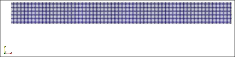
Fig. 2: Baseline Mesh (two-dimensional sliced view)

Mesh 1:

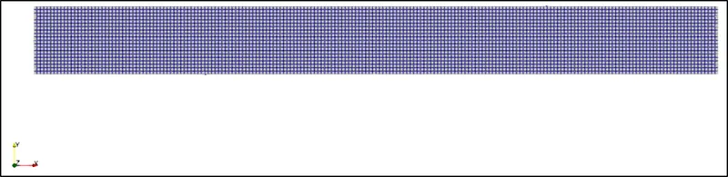
Fig. 3: Mesh 1 (two-dimensional sliced view)

Mesh 2:

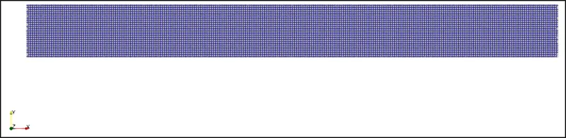
Fig. 4: Mesh 2 (two-dimensional sliced view)

Mesh 3:

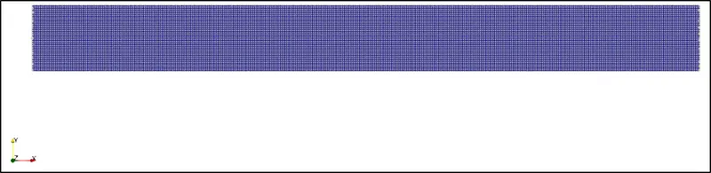
Fig. 5: Mesh 3 (two-dimensional sliced view)

Flow-field parameters	Baseline Mesh	% var	Mesh 1	% var	Mesh 2	% var	Mesh 3	% var
Static Pressure (`P_2`) (Pa)	226895.6	--	227174.8	0.123	226957.3	-0.0957	226450.1	-0.2235
Density (`rho_2`) (`(kg)/m^3`)	2.110478	--	2.106644	-0.181665	2.098868	-0.3691	2.088454	-0.4962
Temperature (`T_2`) (K)	373.1562	--	374.21	0.2824	375.029	0.21886	375.6914	-0.1766
Velocity (`u_2`) (`m/s`)	214.2475	--	214.6683	0.1964	214.3306	-0.1573	213.4134	-0.4279

Table 6: Percentage variation in values of flow-field parameters for different mesh configurations (Data highlighted in bold indicates the least value of percentage variation for that parameter)

Flow-field parameters	Analytical Solution	Baseline Mesh	% error	Mesh 1	% error	Mesh 2	% error	Mesh 3	% error
Static Pressure (`P_2`) (`Pa`)	231968.0409	226895.6	-2.1867	227174.8	-2.0663	226957.3	-2.1601	226450.1	-2.3787
Density (`rho_2`) (`(kg)/m^3`)	2.091657151	2.110478	-0.8898	2.106644	0.7165	2.098868	0.3447	2.088454	-0.1531
Temperature (`T_2`) (K)	386.341304	373.1562	-3.4128	374.21	-3.14	375.029	-2.928	375.6914	-2.7566
Velocity (`u_2`) (`m/s`)	220.3954978	214.2475	-2.7895	214.6683	-2.5986	214.3306	-2.7518	213.4134	-3.16798

Table 7: Percentage error comparison between predicted values of flow-field parameters for different mesh configurations and their analytical solutions (Data highlighted in bold indicates the least value of percentage error for that parameter)

Time statistics and Mesh quality attributes for the different mesh configurations:

Mesh	Total Cells	Run Time [s]	Max Aspect Ratio	Max Skewness	Max Non-Orthogonality
Baseline	40960	83.95796	~1	1.17578e-38	1.17578e-38
1	80000	232.68278	~1	1.17578e-38	1.17578e-38
2	168000	481.63311	~2	1.17578e-38	1.17578e-38
3	319488	1321.45498	~2	1.17578e-38	1.17578e-38

Table 8: Time statistics and Mesh quality attributes depicting the maximum values of aspect ratio, skewness and non-orthogonality for different mesh configurations of the shock tube domain consisting of two different pressure regions, initially separated by a diaphragm

From the meshing statistics in Table 6, it can be seen that across different mesh configurations, only temperature as a flow-field quantity represents a consistently decreasing percentage variation in values with every subsequent mesh refinement whereas the remaining quantities viz., static pressure, density and velocity are unsteady. This resulted in averaging the values of the static pressure, density and velocity quantities for all the meshes and determining the mesh whose difference would be the least from the mean leading to mesh 2 with 168000 cells as an overall best fit which was accordingly deemed to be the mesh independent result, also in terms of the computational time and resources. It should be noted that the values predicted for all the aforementioned quantities by each mesh were averaged over the corresponding range to which they belonged as opposed to finding the minimum or maximum values for the same. The % var is calculated as the ratio of the difference of the predicted values in two consecutive meshes to the predicted value of the previous mesh e.g., ((Density for Mesh 2 - Density for Mesh 1)/Density for Mesh 1). Similarly, mesh number 3 (or mesh 3) with 319488 cells represents the least value of percentage error in prediction for density and temperature parameters, which again is steadily decreasing with every subsequent mesh refinement when compared against the analytical solution, as seen in Table 7, however, the static pressure and velocity quantities are fluctuating when considered from the same perspective. With that being said, the difference in percentage error does not drastically change as much as the resultant increase in computational resources and therefore, the same mesh 2 configuration can also be considered to have been validated against the analytical solution as the percentage difference in accuracy between them is under 3% (negative sign only denotes the deviation with respect to the analytical solution) for all of the previously mentioned flow-field parameters. Additionally, mesh quality attributes of all the different meshes prepared in Table 8 indicates that they lie in the range of acceptable values and remains constant, almost tending to ideal values , for skewness and non-orthogonality, as previously stated in Table 1, as well as for aspect ratio with regards to the Baseline mesh and mesh 1 but slightly deteriorates for mesh 2 and mesh 3 while again remaining constant which may be attributed to a significant increase in the number of mesh cells within the same confined regions. Results in Section 3 dealing with visualisation of flow-field parameters using field plots will only be referred with regards to the mesh independent solution i.e., Mesh 2.

2.4 Post-Processing

The extended part of the solution process using Converge Studio v3.0 included selecting the variables of interest whose quantitative and qualitative aspects would highlight the behaviour of the flow, in this case within the given fluid domain, under different circumstances and they were chosen by clicking on the 'Post variable selection' sub-option of the 'Output/Post-Processing' setting under the 'Case Setup' tree and checking the boxes 'Density', 'Mesh Quality', 'Pressure', 'Temperature', and 'Velocity' in the 'Typical Variables' section and 'Region ID' (normally enabled by default) in the 'Geometry/Location' section of the 'Typical Variables/Geometry' tab and adding 'Mass Fraction' under 'Species' section of the 'Species/Passive' tab for `O_2` and `N_2` species with respect to the concerned numerical analysis. Visualising the different flow variable quantities in two-dimensional space in ParaView required the creation of a slice of the given fluid domain by using the "Slice" tool in the 'Commons' toolbar typically located above the 'Pipeline Browser' window based on default layout settings and choosing 'Z Normal' under 'Plane Parameters' section to align the plane normal to the z-axis direction such that the entire domain was viewed in the direction of flow followed by unchecking the 'Show Plane', 'Triangulate the slice' and 'Merge duplicated points in the slice' boxes for disabling the viewing of the plane borders, production of triangles in the output and overlapping data points respectively. Plotting the velocity, temperature, pressure and density profiles across the given domain for both the verification and validation cases were performed by using ParaView's in-built "plot over line" tool. The "plot over line" tool was accessed by clicking on 'Filters' present in the data analysis group, followed by entering the coordinates as seen in Table 9 before clicking on the "Apply" button to view the said profiles.

It was ensured that the last time-step size of the simulation run was selected to view the velocity magnitude, temperature, pressure and density profile results. Additionally, velocity magnitude, pressure, temperature and density field plots were created to view the development of the flow field characteristics across the fluid domain at different time intervals. Legends, titles, and x and y labels were added for better understanding of the graphical representations.

Line 1	x	y	z
Point 1	-2.5	0	0
Point 2	7.5	0	0

Table 9: Line Coordinates for viewing the velocity magnitude, temperature, pressure and density profiles across the domain

To save an animation file of the different field plots, the option 'Save Animation' was accessed under the 'File' menu and clicked on followed by choosing the appropriate settings under the different sections such as 'Size and Scaling', 'Coloring', 'Compression Options' and 'Animation Options' to name a few, assigning an appropriate name to the animation file, in this case by the variable whose field plot is being indicated before clicking on the 'OK' button.

2.6 Convergence Level

In the given numerical analysis, transient simulations using first-order implicit Euler time advancement scheme were performed to accommodate for larger time-steps while also being numerically stable along with a Density-based solver, to account for the compressibility effects, of type modified Pressure Implicit with Splitting of Operator (PISO) which is an iterative pressure-velocity coupling algorithm involving a predictor step for predicting solution of the momentum equation from which a pressure equation is obtained and solved whose correction is then consequently reapplied to the momentum equation such that this process continues until the desired level of accuracy is achieved. At the end of the momentum predictor and first corrector step, remaining transport equations were solved in series. In other words, momentum and pressure are solved at the first PISO iteration which enables calculation for velocity terms required by other transport equations and at the end of each iteration in the PISO loop, convergence criterion is checked for which in the case of compressible flow (Mach number in regards to the shock wave velocity of 503.7847m/s (See Section 2.3.4 Mesh Refinement approach and selection of transient parameters for the given numerical simulation) results in an approximate value of 1.45 which is much higher than the typical range of 0.2 to 0.3 and as such the compressibility effects are needed to be considered) requires the density correction error term to be less than the value of PISO tolerance which remains unchanged for the given numerical simulation at its default value of 1e-03. The selection of solver types for the different equations within 'Solver parameters [Transient]' sub-option in the 'Simulation Parameters' settings under the 'Case Setup' tree included assigning SOR to Momentum, Pressure, Density and Energy equations. The SOR solver type is a generally preferred algorithm owing to its advantage in being computationally less expensive than the different forms of biconjugate gradient stabilized (BiCGSTAB) algorithms or HYBRID (wherever applicable). The solver types, convergence tolerance limits, and minimum and maximum iterations defined for the equations corresponding to the default physical model and the monitor variable plots corresponding to the different mesh configurations are shown in the table and figures below:

Equations	Solver Type	Convergence Tolerance	Minimum Iterations	Maximum Iterations	Preconditioner
Momentum	SOR	1e-05	2	50	None
Pressure	SOR	1e-08	2	5000	None
Density	SOR	1e-04	2	20	None
Energy	SOR	1e-04	2	20	None

Table 10: Solver Types, Convergence Tolerance Values, Minimum and Maximum Iterations and Preconditioners of the different equations used in the default physical model

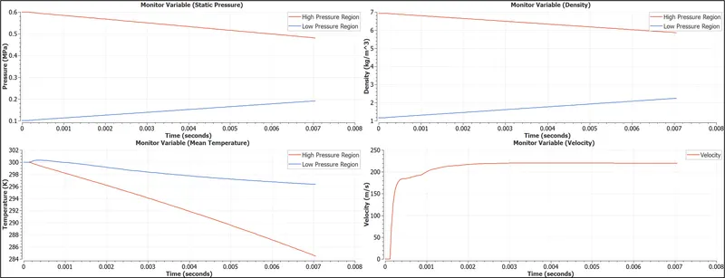
Fig. 10: Plots of monitor variables density, pressure and mean temperature for the 'High Pressure' and 'Low Pressure' regions and increase in velocity across the contact surface of the given shock tube domain using transient simulation for the baseline mesh

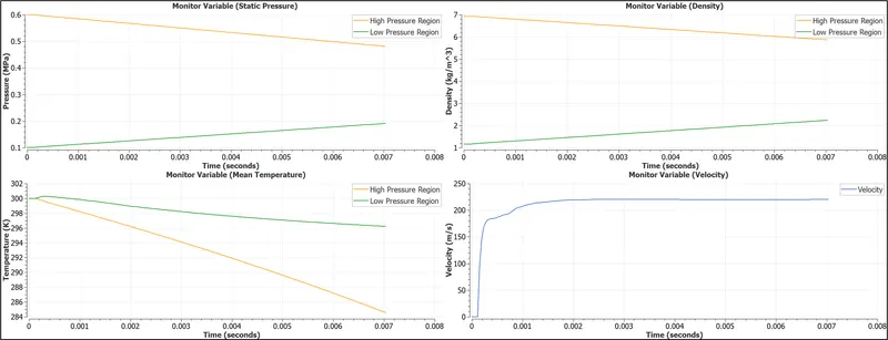Fig. 11: Plots of monitor variables density, pressure and mean temperature for the 'High Pressure' and 'Low Pressure' regions and increase in velocity across the contact surface of the given shock tube domain using transient simulation for the mesh 1

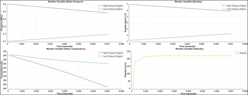
Fig. 12: Plots of monitor variables density, pressure and mean temperature for the 'High Pressure' and 'Low Pressure' regions and increase in velocity across the contact surface of the given shock tube domain using transient simulation for the mesh 2

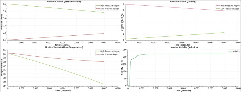
Fig. 13: Plots of monitor variables density, pressure and mean temperature for the 'High Pressure' and 'Low Pressure' regions and increase in velocity across the contact surface of the given shock tube domain using transient simulation for the mesh 3

From Fig. 10, Fig. 11, Fig. 12 and Fig. 13, it can be observed that the monitor variables for static pressure, density and mean temperature provide nearly consistent values as time progresses in both the 'High Pressure' and 'Low Pressure' regions while velocity across the contact surface, which is the zone between the concerned regions after the diaphragm is immediately broken, appears to have achieved convergence in regards to attaining a steady state value which was initially at 0m/s.

3. Results

3.1 Velocity magnitude, density, static pressure and temperature values using field plots

Fig. 14 to Fig. 17 below shows the velocity magnitude, density, static pressure and temperature values for mesh independent result, mesh 2, across the shock tube domain consisting of high and low pressure regions separated by a diaphragm, which gets broken at t = 0.0001s, in two-dimensional space using field plots at the slice region created by orienting the plane normal to the flow direction as was specified in Section 2.4 Post-Processing. It can be observed that the moment the diaphragm gets broken, discontinuous propagation of flow-field properties occurs across the contact surface i.e., the interface between the "Driver" and "Driven" gas regions, such that a normal shock wave is generated which travels towards the "Driven" gas region with a certain shock wave velocity, consequently increasing the pressure immediately behind it, along with giving rise to mass-motion velocity which also becomes the new travelling speed for the contact surface while an expansion wave gets created in the direction of the "Driver" gas region such that its initially high pressure gets gradually reduced behaving similar to isentropic flow conditions. The remaining properties, density and temperature, can be visualised in the same context as pressure and velocity quantities based on the flow characteristics developing within the shock tube.

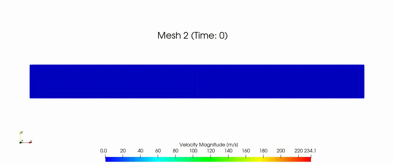
Fig. 14: Velocity Magnitude field plot across the domain for mesh 2 in two-dimensional space

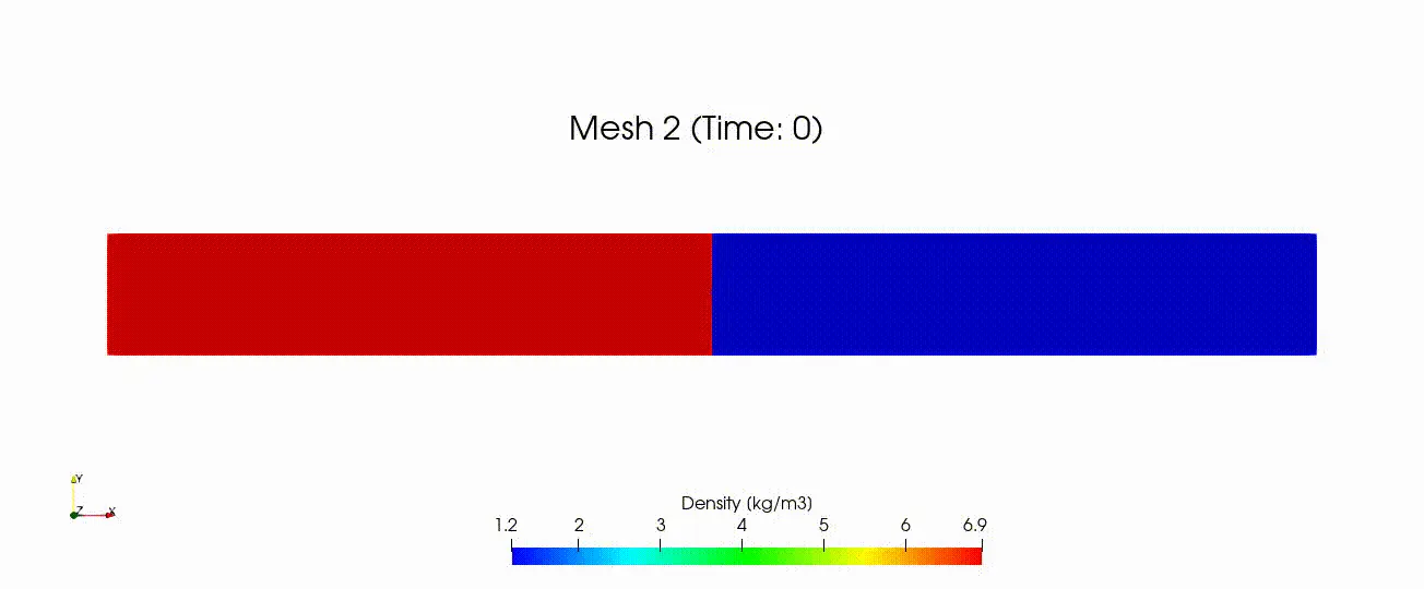
Fig. 15: Density field plot across the domain for mesh 2 in two-dimensional space

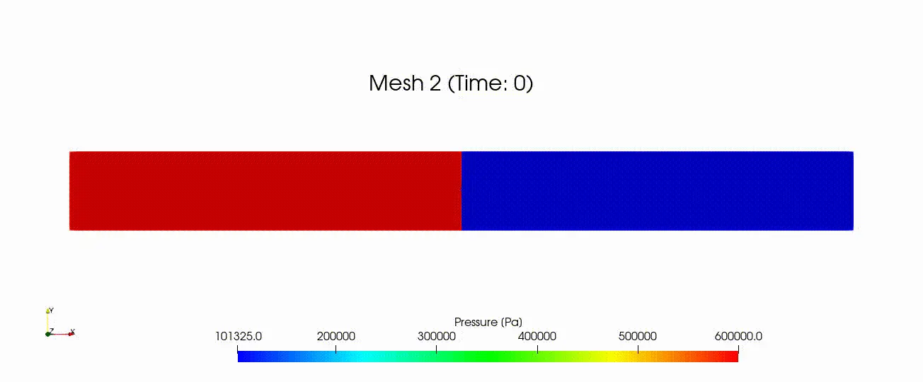
Fig. 16: Static pressure field plot across the domain for mesh 2 in two-dimensional space

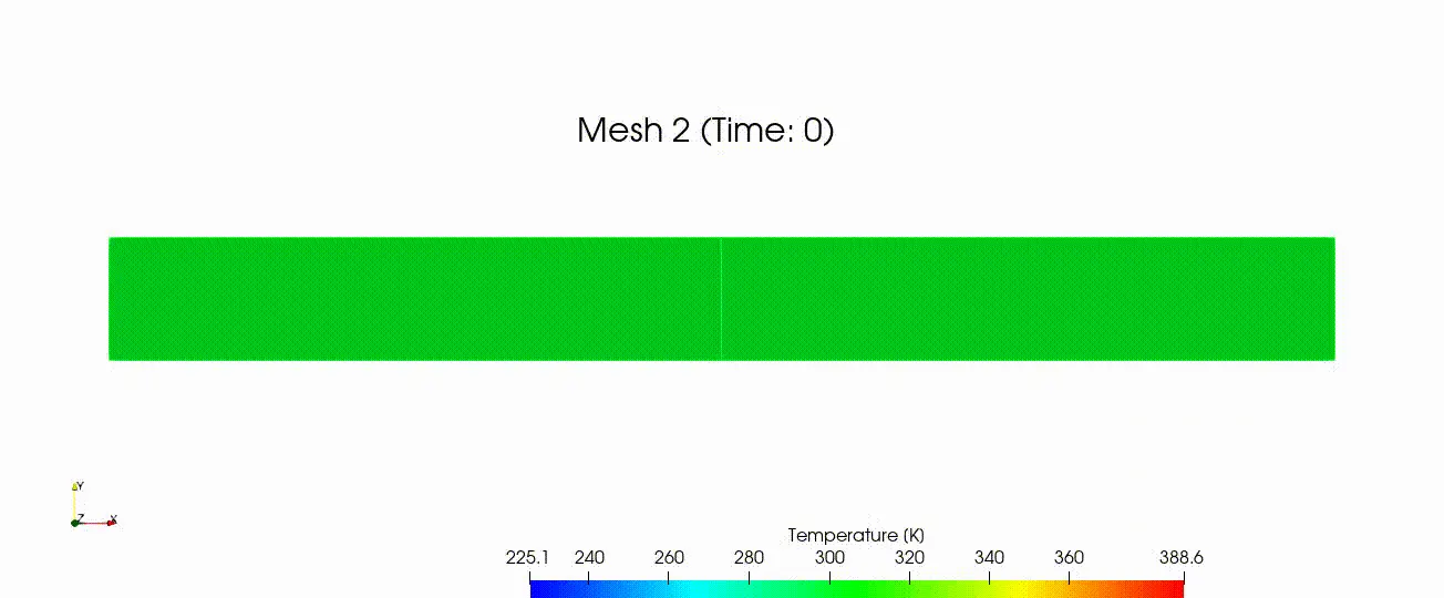
Fig. 17: Temperature field plot across the domain for mesh 2 in two-dimensional space

3.2 Velocity magnitude, density, static pressure and temperature values using line plots

Fig. 18 below shows the comparison between the flow-field properties of unsteady wave motion within a shock tube at time t = 0.007s predicted by different mesh configurations and the analytical solution for the same setup wherein with every subsequent mesh refinement, the differences become smaller, or in other words the numerical solution improves in agreement against its counterpart analytical solution profiles when the concerned regions are allowed to significantly develop with respect to the domain length. There are, however, noticeable disagreements especially when a change occurs at the onset and towards the end of different regions like the shock front and expansion wave and these may be due to the gradients of different flow properties specific to these regions requiring more or better quality cells to capture the same.

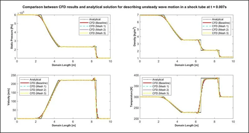
Fig. 18: Comparison between CFD results using different mesh configurations and analytical solution of different flow properties describing unsteady wave motion within a shock tube at t = 0.007s

4. Discussion

Air, containing a mixture of two major contributing gas species `O_2` and `N_2` by mass fraction, is initially separated into two regions viz., high pressure, "Driver", on the left hand side with respect to the viewing plane and low pressure, "Driven", on the right hand side, by a diaphragm located at mid-point position of 5m with respect to the length of the shock tube domain which is closed at either ends. Fluid flow across the shock tube domain does not take place until a designated time at which the diaphragm gets broken after which it remains essentially parallel and unaffected with respect to the walls bounding it which are of the type "slip" condition such that the effects of viscosity are negligible or quite simply the flow can be described as inviscid which is in line with the modelling considerations made for this numerical study. The breaking of the diaphragm leads to the generation of a shock wave, which gets transmitted towards the "Driven" section, and an expansion wave disseminated towards the "Driver" section. The shock wave travelling in the direction of the "Driven" section causes increase in the pressure of the gas immediately behind it followed by the creation of mass-motion velocity such that the contact surface, which is essentially the interface between the "Driver" and "Driven" gases, also travels at this particular velocity while the entropy across it changes erratically. Also, visualising the shock wave as moving instead of stationary provides further insights into properties such as total enthalpy which is not constant across it and as a result determining other parameters such as temperature and density would no longer depend on the Mach number but a more characteristic attribute like pressure ratio. The flow properties such as pressure and velocity across the contact surface, however, are preserved. As for the expansion wave, the flow behaviour is such that the change in properties does not occur abruptly but rather gradually resembling isentropic conditions with pressure, density and temperature decreasing in this zone of the "Driver" section.

5. Conclusion

The numerical analysis for three-dimensional, transient state simulations of air flow movement across the shock tube domain consisting of high and low pressure regions separated by a diaphragm, which gets broken at t = 0.0001s, using the default physical model in Converge Studio v3.0 and executed using the Cygwin64 terminal was well understood. It was realised that implementing the "Events" feature of CONVERGE for the given numerical study allowed both a time-based and region-based control for flow to be initially prevented and then to take place thereby greatly improving the visualisation of the unsteady wave motion. Moreover, the different base grid size settings with regards to mesh refinement indicated improved agreement with the analytical solution, however, a different meshing approach that would capture the gradients better at the onset and towards the end of both the shock front and expansion wave regions is required to be investigated and is under consideration from a future scope of study.

References

[1] John D. Anderson, Jr., (2003). Modern Compressible Flow With Historical Perspective (Eds.), Unsteady Wave Motion (3rd ed., pp. 261–302). McGraw-Hill.

[2] CONVERGE 3.0 Manual. © 2020 Convergent Science. All rights reserved. July 15, 2020.

[3] The Engineering Mindset, Properties of Air at atmospheric pressure, https://theengineeringmindset.com/, viewed 17 August 2021, <https://theengineeringmindset.com/properties-of-air-at-atmospheric-pressure/>

[4] Celik, I. , Ghia. U., Roache, P., Freitas, C., Coleman, H., Raad, P., "Procedure for Estimating and Reporting of Uncertainty Due to Discretization in CFD Applications," American Society of Mechanical Engineers Journal of Fluids Engineering, Vol. 130, July 2008.