Week 11 - Simulation of Flow through a pipe in OpenFoam
1. Introduction
Flow through a bounding solid surface in which the fluid completely occupies the volume across it such that the flow is driven as a result of the pressure gradient can be described as internal flow. Heating and cooling applications involving the use of fluid flow through pipes, flow in arteries and veins are some of the common examples of internal flow. The aim of this challenge was to perform a two-dimensional transient axi-symmetric numerical simulation of an incompressible-laminar-viscous flow using the wedge boundary condition across a pipe of constant cross-section with flow characteristics resembling inlet conditions at Reynold's number of 2100. The objectives also include validation of results obtained with the Hagen-Poiseuille's equations for the fully developed flow and preparation of a MATLAB script to automate the generation of the blockMeshDict file by taking input variables like pipe diameter and wedge angle.
2. Method
The typical approach adopted to performing numerical simulation in OpenFOAM involves the following steps:
- Identifying the tutorial in the 'FOAM_TUTORIALS' folder that contains the appropriate governing equations relevant to the physics of the flow for the given problem. A typical file structure of an OpenFOAM tutorial consists of the below mentioned directories and files:
- A 'system' directory with the 'controlDict', 'fvSchemes' and 'fvSolution' files used for specifying the numerical schemes and solution procedure along with control on the simulation run properties. Additionally, for the given numerical problem, a file by the name 'blockMeshDict' mentions the creation of a hex block representing the geometry as well as its mesh properties.
- A 'constant' directory that contains a 'polyMesh' directory outlining the various aspects of the mesh such as 'boundary', 'points', 'faces', etc., and a file that defines the physical properties, in this case, 'transportProperties' specifying the value of kinematic viscosity.
- A time directory, usually called the '0' directory that consists of files representing the different fields or fluid flow properties with values as required at the start of simulation run or at time `t = 0`.
- Copying the now identified tutorial folder from the 'FOAM_TUTORIALS' folder to the 'FOAM_RUN' folder, specifically created to allow simulation run of OpenFOAM numerical simulation cases, with either the same name or preferably a name relevant to the geometry to be discretized.
- Replacing the geometry and boundary list of the pre-existing tutorial with the geometry and boundary list pertaining to the given problem and defining mesh parameters with regards to the flow physics, in this case by updating the 'blockMeshDict' file (Section 2.1 Modelling).
- Updating the 'transportProperties' file with kinematic viscosity value of water at 25°C (Section 2.2 Evaluation of inlet velocity from Reynolds number and entrance length).
- Updating the fields' files present inside the '0' directory viz., 'U' and 'p', with the boundary list as specified in the 'blockMeshDict' file and appropriate values at the relevant boundary to ensure the given numerical problem has the right boundary conditions and that the solution would be correctly initialised (Section 2.3 Boundary Conditions).
- Updating the 'controlDict' file, in this case the 'deltaT' and 'endTime' parameters with values that take into consideration domain specific attributes such as length of the pipe in the direction of flow, fluid flow velocity and avoiding violation of Courant-Friedrichs-Lewy Condition or the CFL number by limiting its mean and maximum value during simulation run below 1 (Section 2.5 Determination of transient parameters).
The above steps were executed using Linux commands in a Ubuntu 20.04.2.0 LTS (Long Term Support) operating system as shown below:
i) Change directory to FOAM_RUN:
cd $FOAM_RUN
ii) Copy cavity example from FOAM_TUTORIALS directory that contains the icoFoam solver to the FOAM_RUN directory:
cp -r $FOAM_TUTORIALS/incompressible/icoFoam/cavity/cavity .
iii) Rename cavity directory to Week_11_flow_through_pipe_simulation
mv cavity Week_11_flow_through_pipe_simulation
iv) Change directory to Week_11_flow_through_pipe_simulation
cd Week_11_flow_through_pipe_simulation
v) Replacing the geometry and boundary list by editing the 'blockMeshDict' file:
gedit system/blockMeshDict
vi) Updating the kinematic viscosity value by editing the 'transportProperties' file:
gedit constant/transportProperties
vii) Updating the boundary list and boundary conditions by editing the 'U' and 'p' files:
gedit 0/U
gedit 0/p
viii) Updating the 'deltaT' and 'endTime' parameters with appropriate values by editing the 'controlDict' file:
gedit system/controlDict
ix) Creating the block based geometry and generating mesh for the computational domain:
blockMesh
x) Running the icoFoam solver to solve for the incompressible laminar Navier-Stokes equations:
icoFoam
xi) Post-processing and visualising results of the performed simulation (Section 2.5):
paraFoam
2.1 Modelling
The problem was solved by constructing a single three-dimensional hexahedral block (number of mesh elements in y-direction was set to 1 for a two-dimensional axi-symmetric flow problem) that resembled a cut-section of the pipe, similar to an elongated wedge (as seen in Fig. 1), whose angle with the centre (or the wedge angle) was less than 5°, in this case at 4°, with the block defined using 6 vertices by collapsing its bottom face or in other words, merging vertices on the bottom side of the front and back faces that were adjacent to the bottom face, in a dictionary type file called 'blockMeshDict' (file snippet for which is attached below with this report). Vertices were assigned in which the origin, or point '0', was selected as the first point lying along the axis of symmetry. The line stating the creation of hex block in the 'blockMeshDict' file followed the arrangement of vertices according to the right-hand system such that the normal (direction in which the thumb of the right hand pointed towards) was oriented outwards or along the positive z-axis direction for the surface containing vertices 3, 2 and 5 implying the vertices were to be numbered along which the remaining fingers of the right hand curled towards, i.e., in counter-clockwise direction to the positive z-axis direction. The principle remained the same for defining the faces of the boundaries in the 'boundary' section of the 'blockMeshDict' file, only this time the normals would face outwards from each of the respective surfaces such that the region defining the 'inlet' would have its normal facing outwards in the negative z-axis direction, 'outlet' with normal in the positive z-axis direction, top wall surface of the domain with normal in the positive x-axis direction, front surface of the domain with normal in the positive y-axis direction and back surface of the domain with normal in the negative y-axis direction while vertices would be numbered in a similar manner again along the direction in which the remaining fingers of the right hand curled towards for each of the regions mentioned previously. The total number of grid points along the z-axis and x-axis directions have been so taken that a cell is created at every 0.0001m and 0.000142857m respectively or in other words, number of cells along the longer z direction is 1200 while number of cells along the x direction is 35. A hex block definition also consists of specifying the cell expansion ratios, in this case along each local cartesian coordinate direction using 'simpleGrading', which equates to the ratio of the width of the end/last cell to the width of the start/first cell along the same edge of a particular block. For the given numerical simulation, a cell expansion ratio of 1 was chosen which indicates that the width of the end/last cell is equal to the width of the start/first cell. Since, the given domain has been reduced from a pipe of circular cross-section, on the basis of axi-symmetric flow conditions, for improving the computational performance of the numerical simulation with regards to increased grid density and reduced computational time, the pair of vertices (1,4) and (2,5) were accounted as the curvature areas of the pipe from which they were extracted by specifying the 'arc' in 'edges' keywords connecting these pair of vertices that followed through their interpolation points, in this case represented by the radius of the pipe at the x-coordinate for both while the z-coordinate for the former pair at 0 and the latter pair at a distance equivalent to the pipe length. It should be noted that due to the small value of the wedge angle, the 'arc' for the pair of vertices (1,4) and (2,5) was almost visualised as an approximated straight line. The meshing approach adopted for the given computational domain was developed to maintain the meshing quality attributes viz., aspect ratio, skewness and non-orthogonality, within the ranges outlined by CFD support [1] in the following table:
|
Aspect Ratio |
1 - Best possible value | ||
|
Skewness |
<20 although higher values affect the accuracy of results |
||
|
Orthogonal Quality |
n0<70 (Safe Values) |
70<n0<90 (requires special treatment) |
n0>90 (unacceptable) |
Table 1: Mesh Quality Attributes as defined by CFD support [1]
The reason for targeting the above mentioned mesh quality attributes comes from analysis across different types of flow problems that these are few of the known ways of identifying whether the discretized mesh would develop convergence issues during the solution process and to avoid fatal solver scenarios.
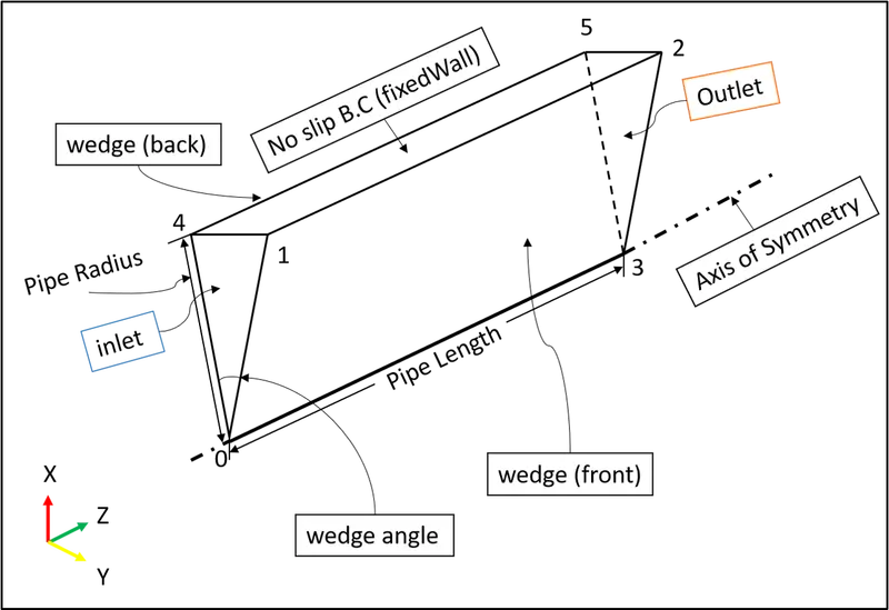
Fig. 1: Pipe flow Geometry (single hexahedral block and vertices representing the decomposed main domain, and boundary conditions)
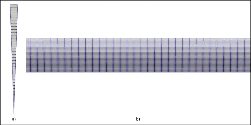
Fig. 2: Baseline mesh domain: a) View from the inlet patch, b) View across the computational domain from the front patch at the middle section of the pipe geometry
2.2 Evaluation of inlet velocity from Reynolds number and entrance length
Reynolds number, based on the inlet pipe diameter, can be expressed below as:
`Re = (U*L)/nu`, where (Eq. 1)
`U` is the inlet velocity,
`L` is the characteristic length, in this case, the inlet diameter of the pipe, and
`nu` is the kinematic viscosity of fluid i.e., water at 25°C
Substituting the value of given Reynolds number as 2100, inlet diameter of pipe selected as 0.01m and kinematic viscosity of water at 25°C as 8.9e-7 [2] in (Eq. 1), we get inlet velocity of water flowing through the pipe as 0.1869m/s.
Entrance region determined by the entry length or Hydro-dynamic length is typically considered as the distance from the entrance of the pipe to the position where the wall shear stress assumes about two percent of its fully developed value and is also the point wherein the value of velocity reaches its maximum value at the center of the pipe, in this case at the axis of symmetry, due to the development of a boundary layer more of which has been described in detail under Section 4. Discussion. The entrance length which in the case of laminar flow, in non-dimensional form, can be expressed mathematically as shown below:
`(L_h)/D cong 0.05*Re` (Eq. 2)
Substituting the values of inlet diameter of pipe and Reynolds number in (Eq. 2), the entrance length or Hydro-dynamic length was evaluated to a value of 1.05m from the inlet of the pipe geometry in the direction of flow.
2.3 Boundary Conditions
The different regions of the mesh, identified as patches, that demarcate its extents as well as specify the boundary conditions to be employed on them is written in a list called as 'boundary' in the 'blockMeshDict' file. The input and output data in OpenFOAM are recorded as tensor fields which are written onto time directories, in this case the fields being velocity ('U') and pressure ('p') in the '0' folder, and read from it at an appropriate time. A typical structure of the field data file consists of the 'dimensions' written with 7 scalars representing the 'dimensionSet' enclosed by square brackets with each scalar highlighting the properties of mass, length, time, temperature, quantity, current and luminous intensity respectively from left to right in base units for SI and USCS, 'internalField', in this case of type 'uniform', that allocates a single value to all elements within the field and expressed using 3 vector components for velocity (U) and only 'uniform 0' for pressure (p) as it is kinematic pressure for an incompressible case for which its absolute value is of little significance, and 'boundaryField' which consists of a list of boundary conditions and data for all patches, preferably identical in name to the patches created in 'boundary' in the 'blockMeshDict' file. For the given numerical simulation, the different patch names and patch types of the 'blockMeshDict' file and boundary fields (type and value) of the time directory files, 'U' and 'p' (file snippets for which is attached below with this report), describing the numerical simulation of an incompressible-laminar-viscous flow through the pipe geometry is mentioned in the following table:
|
patch name |
inlet |
outlet |
fixedWall |
front |
back |
axis |
|
patch type (in blockMeshDict) |
patch |
patch |
wall |
wedge |
wedge |
empty |
|
type (in U) |
fixedValue |
zeroGradient |
noSlip |
wedge |
wedge |
empty |
|
value (in U) |
uniform(0 0 0.1869) |
-- |
-- |
-- |
-- |
-- |
|
type (in p) |
zeroGradient |
fixedValue |
zeroGradient |
wedge |
wedge |
empty |
|
value (in p) |
-- |
uniform 0 |
-- |
-- |
-- |
-- |
Table 2: Boundary Conditions and its setup
Type 'zeroGradient' in '0' time directory files, 'U' and 'p', indicates the normal gradient of that particular field at the relevant patch name is 0, type 'noSlip' is used to set the velocity of the 'fixedWall' patch to (0 0 0), type 'wedge' is used in two-dimensional axi-symmetric cases, in this case the pipe representing a cylinder is specified as a wedge of certain angle with the center (usually less than 5°) that is 1 cell (or element) thick extending across the centerline, and type 'empty' for the 'axis' patch is used in two dimensional flow problems indicating that the plane on this surface is normal to the third dimension which requires no solution. In regards to the establishment of keywords such as 'vertices', 'edges', and 'faces' in Section 2.1 Modelling as well as the patches pertaining to the 'boundary' list of the 'blockMeshDict' file from Table 1 above, a MATLAB script (code snippet for which is attached below with this report) was then prepared by taking into account input variables like pipe diameter and wedge angle for automating the generation of the 'blockMeshDict' file.
2.4 icoFoam model
The icoFoam solver uses the PISO pressure-velocity coupling algorithm to solve the incompressible laminar Navier-Stokes equations. The Navier-Stokes equations define the fluid flow properties such as velocity, pressure, density, temperature, viscosity, energy, etc., within a given physical domain. Additionally, the Navier-Stokes equations are developed with regards to the laws of conservation that states the net mass flow across a system is zero (Conservation of mass), momentum within the same system (or control volume) is constant (Conservation of momentum). The continuity and momentum equations are mathematically expressed below as:
Continuity equation: `nabla*U = 0`
Momentum equation: `del/(del t)*(u) + nabla*(uotimesu) - nabla*(nu*nablau) = -nabla p` ; where
`u` is velocity (in m/s), and
`p` is kinematic pressure (in `m^2/s^2`)
2.5 Determination of transient parameters
The setup of simulation run time and time-step size for any given computational domain in OpenFOAM is described in the 'controlDict' dictionary file. Typically, the start of any simulation begins at `t = 0`, in which case OpenFOAM is required to read the field values of the '0' directory and therefore 'startFrom' keyword is set to 'startTime' which is in turn set to 0 referring to the '0' directory. The 'endTime' depends on the domain length and the flow velocity, in the direction of flow, such that the fluid medium passes through it at least 10 times to acquire steady state conditions, in the case of laminar flow as a mark of a general rule and also as a recommendation in the OpenFOAM v8 User Guide. Therefore, 'endTime' can be evaluated as shown below:
`endTime = (L/U)*10`; where (Eq. 3)
`L` is the length of the computational domain = 1.2m, and
`U` is the fluid flow velocity = 0.1869m/s
From Eq. 3, we get value of 'endTime' approximately as 64.205s rounded to the nearest whole number at 65s. Time-step size, 'deltaT' was decided based on the CFL number which is expressed below:
`CFL = (U*Delta t)/(Delta z)`; where (Eq. 4)
`Delta t` is time-step size,
`Delta z` represents the smallest cell size, which was calculated as the ratio of length of the computational domain to the number of mesh elements in the direction of flow, in this case along z-axis direction, i.e.,
`Delta z = L/n_z`; (Eq. 5)
In order to attain temporal accuracy and numerical stability using the 'icoFoam' solver, the CFL criteria was required to be less than 1 and therefore, the value of time-step size was initially determined with the limiting value of the CFL criteria as 1 and tabulated as shown below:
|
`Delta z` (in m) (Eq. 5) |
Time-step size (`Delta t`) (in s) (Eq. 4) |
|
0.001 |
0.00535 |
Table 3: Smallest element size (`Delta z`) and time-step size (`Delta t`) values
The above calculated value of time-step size in Table 3 resulted in the mean Courant number to report values less than 1, however, the maximum Courant number continued to be greater than 1. Therefore, the time-step size was further reduced to 0.00268s as a trade-off between computational time and the maximum Courant number reporting values just under 1 (file snippet for which is attached below with this report).
2.6 Post-Processing
Plotting the velocity profile at the Hydro-dynamic length from the inlet of the geometry was performed by using ParaView's in-built "plot over line" tool. The "plot over line" tool was accessed by clicking on 'Filters' present in the data analysis group, followed by entering the coordinates as seen in Table 4, and then clicking on the "Apply" button to view the said profile. Similarly, the pressure profile across the entire domain was represented using the "plot over line" tool, however, with coordinates as depicted in Table 5. Visualisation of the wall shear stress plot was essentially a four-step process which has been described briefly as follows:
- Determination of the magnitude of velocity (U) using the calculator tool:
- Select the calculator tool from the common toolbar which needs to be enabled, usually selected by default, by accessing the same in the 'Toolbars' option of the 'View' menu.
- Enter an appropriate 'Result Array Name' such as 'mag_U' in the 'Properties' tab of the calculator tool window and select 'mag' (as in Magnitude) item from the 'Scalars' drop-down option in the calculation box followed by round open and close brackets and then 'U' (for Velocity) item from the 'Vectors' drop-down option such that the text reads 'mag(U)' before clicking on the 'Apply' button.
- Evaluate the gradients for magnitude of velocity (U) using the 'Gradients of unstructured data set' tool:
- Select the 'Gradients of unstructured data set' tool by either typing the same in the search window enabled by pressing 'Ctrl+Space' on the keyboard or through the search option from the 'Filters' menu.
- Type an appropriate 'Result Array Name' such as 'grad_mag_U' in the 'Properties' tab of the 'Gradients of unstructured data set' tool window and select 'mag_U' created in point b. of step i., 'Determination of the magnitude of velocity (U) using the calculator tool', as the 'Scalar Array' before clicking on the 'Apply' button after which the 'grad_mag_U' quantity would appear inside the Field Variable selection box.
- Computing the wall shear stress variable:
- Repeat all the steps in point i., 'Determination of the magnitude of velocity (U) using the calculator tool', however ensuring that the 'Result Array Name' is typed as tau (representing wall shear stress) and the calculation box appears as 'grad_mag_U*0.00089' which was entered by selecting 'grad_mag_U' from the 'Vectors' drop-down option followed by multiplying it with the value 0.00089 which is the dynamic viscosity of water at 25°C (expressed in kg/ms) before clicking on the 'Apply' button after which this quantity like the 'grad_mag_U' quantity from point ii., 'Evaluate the gradients for magnitude of velocity (U) using the 'Gradients of unstructured data set' tool', would appear inside the Field Variable selection box.
- Plotting wall shear stress:
- Using the "plot over line" tool as mentioned previously in this section, wall shear stress was plotted at the same coordinates as that of the velocity profile in Table 4.
It was ensured that the last time-step size of the simulation run was selected to view the velocity, pressure and wall shear stress profile results. In order to compare numerical simulation results of velocity and wall shear stress profiles against its analytical counterparts for validation, following expressions were created, one at a time, in the calculation box of the calculator tool with the term on the left-hand side of both the equations as the 'Result Array Name' in the 'Properties' tab of the same tool before plotting them at the coordinates as seen in Table 4:
Expressions:
Analytical Velocity Profile:
U(r)_analytical = 2*0.1869*(1-((coordsX)^2/(0.005^2)))
Analytical Wall Shear Stress Profile:
tau_analytical = 0.00089*2*0.1869*(1-((2*coordsX)/(0.005^2)))
Additionally, velocity (U) and pressure (p) field plots were created to view the development of the flow field characteristics across the fluid domain. Legends, titles, and x and y labels were added for better understanding of the graphical representations.
|
Line |
x |
y |
z |
|
Point 1 |
0 |
0 |
1.05 |
|
Point 2 |
0.005 |
0 |
1.05 |
Table 4: Line Coordinates for viewing the velocity and wall shear stress profiles
|
Line |
x |
y |
z |
|
Point 1 |
0.0025 |
0 |
0 |
|
Point 2 |
0.0025 |
0 |
1.2 |
Table 5: Line Coordinates for viewing the pressure profile
2.7 Mesh Refinement approach
In this numerical simulation, verification of calculation was carried out in the form of mesh independence study to compare the results obtained from the numerical simulation as accurately as possible against the analytical solution for which it was decided to refine the mesh along the radial direction, as the gradients of velocity and wall shear stress varied strongly from the wall towards the axis of symmetry, with the mesh element size being reduced by 20% to minimize errors due to numerical diffusion.
Mesh 1:
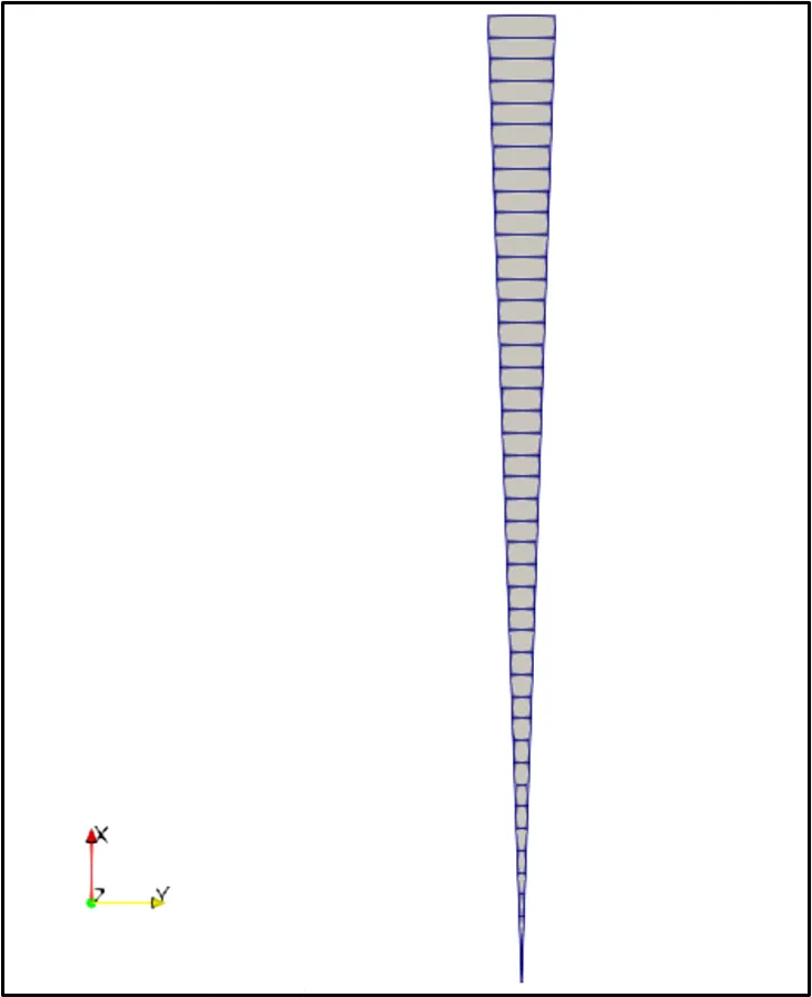
Fig. 3: Mesh 1 (View from inlet)
Mesh 2:
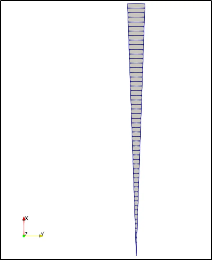
Fig. 4: Mesh 2 (View from inlet)
Mesh 3:
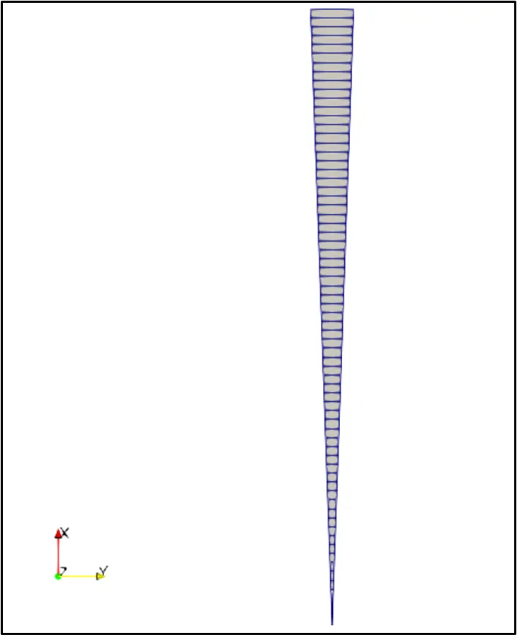
Fig. 5: Mesh 3 (View from inlet)
Mesh 4:
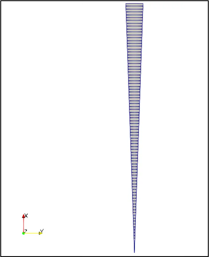
Fig. 6: Mesh 4 (View from inlet)
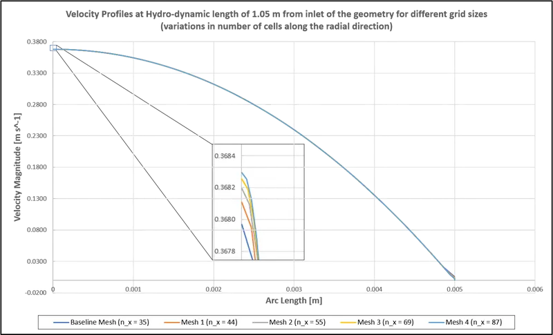
Fig. 7: Velocity Profiles at Hydro-dynamic length of 1.05m from inlet of the pipe geometry for different grid sizes (variations in number of cells along the radial direction)
Mesh and time statistics, and peak velocity magnitude values at the Hydro-dynamic length for different meshes:
|
Mesh |
Number of cells in radial direction (n_x) |
`Delta x` [m] |
Cells |
Execution Time [s] |
Clock Time [s] |
Peak Velocity Magnitude [m s^-1] |
%var |
|
Baseline |
35 |
0.000142857 |
42000 |
3850.84 |
3855 |
0.36796 |
-- |
|
1 |
44 |
0.000113636 |
52800 |
5311.03 |
5312 |
0.368107 |
0.03995 |
|
2 |
55 |
0.0000909091 |
66000 |
7426.98 |
7429 |
0.368194 |
0.02363 |
|
3 |
69 |
0.0000724638 |
82800 |
10162.2 |
10169 |
0.368253 |
0.01602 |
|
4 |
87 |
0.0000574713 |
104400 |
16500.1 |
16505 |
0.368294 |
0.01113 |
Table 6: Mesh and time statistics, peak velocity magnitude values at the Hydro-dynamic length for different meshes, and percentage variation values with subsequent mesh
Mesh quality attributes for the different meshes:
|
Mesh |
Max Aspect Ratio |
Max Skewness |
Max Non-Orthogonality |
|
Baseline |
14.0084 |
0.331709 |
0 |
|
1 |
17.6106 |
0.331709 |
0 |
|
2 |
22.0132 |
0.331709 |
0 |
|
3 |
27.6166 |
0.331709 |
0 |
|
4 |
34.8209 |
0.331709 |
0 |
Table 7: Mesh quality attributes depicting the maximum values of aspect ratio, skewness and non-orthogonality for the different meshes of the pipe geometry
From the meshing statistics in Table 6, mesh number 3 (or mesh 3) with 82800 cells represents a mesh independent result in terms of the computational time (both execution time and clock time) required to achieve a difference in prediction of peak velocity magnitude values by 0.01113%. The %var is calculated as the ratio of the difference of the predicted values in two consecutive meshes to the predicted value of the previous mesh e.g., ((Peak Velocity Magnitude for Mesh 2 - Peak Velocity Magnitude for Mesh 1)/Peak Velocity Magnitude for Mesh 1). Mesh quality attributes of all the different meshes prepared in Table 7 indicates that while the maximum aspect ratio increases as more cells begin to occupy the boundary layer region which does impact the convergence speed as is also seen from Table 6 with both the clock and execution times rising, the maximum skewness and non-orthogonality values remain unaltered due to the quality of cells across the domain continuing to remain of the type hexahedra and prisms and with the number of cells in the case of the former type (hexahedra) increasing with every mesh refinement while the latter type (prisms) remaining constant at 1200. It should be noted that the time-step size (`Delta t`) values were slightly altered from 0.00268s, as reported in Section 2.5 Determination of transient parameters, during the mesh independence study in order to retain the maximum Courant number across the simulation run to be just under 1. Results in Section 3 has been referred with regards to the mesh independent solution i.e., Mesh 3.
3. Results
3.1 Validating the Hydro-dynamic length and fully developed flow velocity profile with the numerical results
Fig.8 below shows the fully developed flow velocity profiles for both the analytical and numerical simulation results at the Hydro-dynamic length of 1.05m from inlet of the pipe geometry. It can be observed that the velocity profile for mesh independent result using number of cells in the radial direction as 69 agrees well with the analytical velocity profile for most parts of the curve length except towards the peak region.
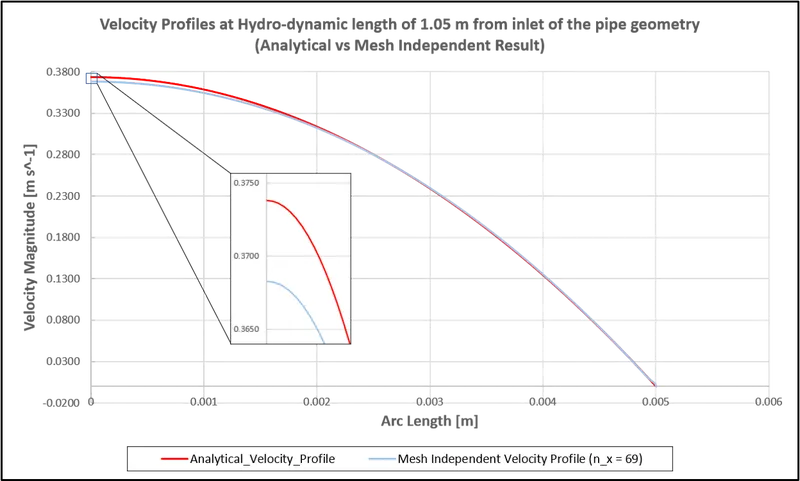
Fig. 8: Velocity profiles at Hydro-dynamic length of 1.05m from inlet of the pipe geometry (Analytical vs Mesh Independent Result)
3.2 Validating the maximum velocity and pressure drop for fully developed flow with the numerical results
Maximum velocity, in the case of fully developed flow laminar flow, is derived from the analytical velocity profile specified in Section 2.6 Post-Processing under Expressions leading to the inference that average velocity is equivalent to one half of the maximum velocity. The expressions for analytical velocity profile and the resulting maximum velocity [3] have been mathematically expressed below as:
Analytical Velocity Profile:
`u(r) = 2*V_(avg)*(1-(r^2)/(R^2))`; where (Eq. 6)
`V_(avg)` is the average velocity, in this case the fluid flow or input velocity `U`,
`R` is the radius of the pipe, and
`r` is the position/coordinate location along the radius of the pipe
Maximum velocity is obtained by substituting `r` as 0 representing centerline position in (Eq. 6):
`u_(max) = 2*V_(avg)` (Eq. 7)
Pressure drop, on the other hand, is demonstrated by the difference in the pressure values across the domain, in this case the pipe geometry, and can be expressed mathematically with regards to the Hagen- Poiseuille's equations for the fully developed flow as shown below:
`Delta P = (32*mu*L*V_(avg))/(D^2)`; (Eq. 8)
It should be noted that the pressure drop expressed in (Eq. 8) has S.I units of the form [kg m s^-2] while pressure values recorded by OpenFOAM with the icoFoam solver has S.I units of the form [m^2 s^-2] representing kinematic pressure as was also mentioned in Section 2.3 Boundary Conditions and Section 2.4 icoFoam model. Therefore, to compare the computed pressure drop from numerical simulation against the analytical solution reported in Table 9, pressure drop in (Eq. 8) was divided by the density of water at 25°C equivalent to 997 (kg/m^3).
From the maximum velocity values, as seen in Table 8, it can be seen that the deviation was recorded to be 1.484% between the mesh independent result and the analytical solution and therefore it can be said that the values are in close confirmation with each other. However, the pressure drop computed by the numerical simulation varies by 32.644% from the analytical solution for the same in Table 9 and this may be attributed to the accuracy in values of the constants used to evaluate the resulting equation and/or the requirement of a finer grid spacing in the direction of flow although the constraints on computational resources in terms of computational time deemed this value to be a suitable trade-off.
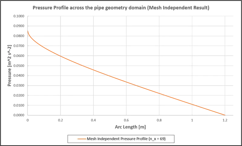
Fig. 9: Pressure profile across the pipe geometry domain for the Mesh Independent Result
|
Maximum Velocity for Analytical Result [m s^-1] (Eq.7) |
Maximum Velocity for Mesh Independent Result [m s^-1] |
% var |
|
0.3738 |
0.368253 |
1.484 |
Table 8: Maximum Velocity values [m s^-1] and percentage variation of the same for Mesh Independent Results from the Analytical solution
|
Pressure Drop for Analytical Result (Eq.8/Density) [m^2 s^-2] |
Pressure Drop for Mesh Independent Result [m^2 s^-2] |
% var |
|
0.06407 |
0.084985 |
32.644 |
Table 9: Pressure drop values [m^2 s^-2] and percentage variation of the same for Mesh Independent Results from the Analytical solution
a) b)
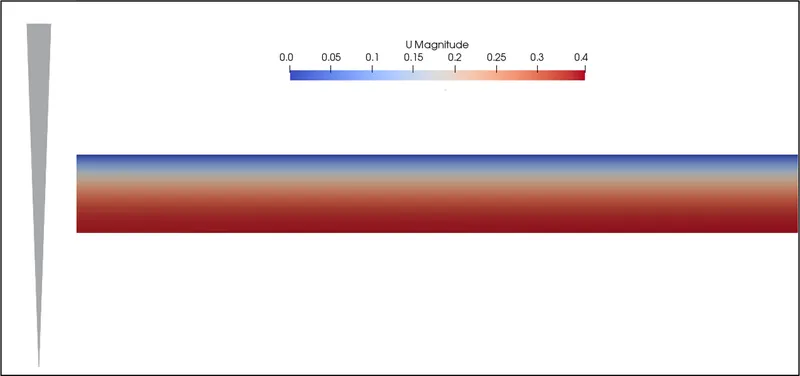
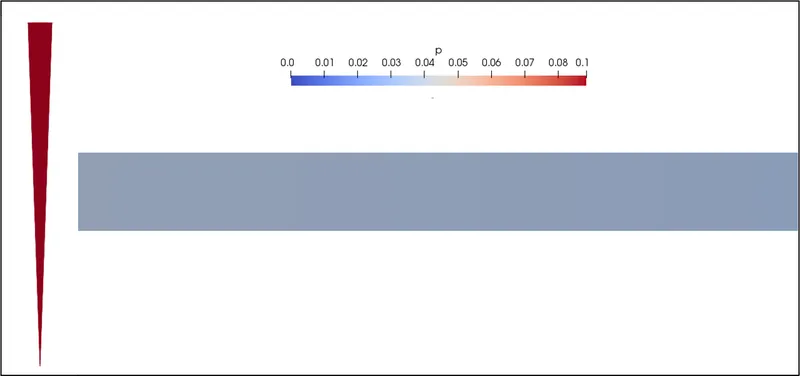
Fig. 10: Field plots at inlet and middle sections of the pipe flow geometry: a) Velocity (U Magnitude) [m s^-1], b) Pressure (p) [m^2 s^-2]
3.3 Validating the wall shear stress for fully developed flow with the numerical results
In Fig.11 below, we can notice the wall shear stress profiles for both analytical and numerical simulation results at the Hydro-dynamic length of 1.05m from inlet of the pipe geometry based on fully developed flow conditions. Similar to the velocity profiles in Fig. 8, it was observed that the wall shear stress profile for mesh independent result using number of cells in the radial direction as 69 agrees well with the analytical wall shear stress profile for most parts of the curve length albeit in certain sections where there are small variations with the maximum deviation between them reported to be a value of 0.03312% near the peak.
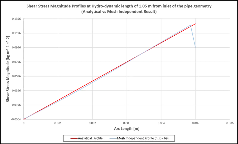
Fig. 11: Wall Shear Stress magnitude profiles at Hydro-dynamic length of 1.05m from inlet of the pipe geometry (Analytical vs Mesh Independent Result)
4. Discussion
The fluid entering the pipe has a uniform profile before it encounters the wall of the pipe and therefore until this point, the flow can be considered as "inviscid" i.e., without the presence of viscous effects. As the fluid progresses downstream from the inlet, it undergoes change when moving along the wall of the pipe as a result of the "no slip" condition and due to the presence of viscous effects, the velocity of flow at the wall surface comes to a value of 0. The flow adjacent to the wall begins to decelerate causing a change in the velocity profile from uniform to a parabolic shape (characteristic of the laminar flow) with every layer from the wall to the center of the pipe increasing in velocity leading to the development of a boundary layer. At the onset of the fully developed flow condition, the velocity profile and wall shear stress represented by the slope of the velocity profile at the wall surface remains unaltered. The highest value of the wall shear stress quantity is typically established at the pipe inlet wherein the boundary layer thickness is the smallest and the value of wall shear stress thereafter decreases gradually as it nears the fully developed flow condition thereby implying that the pressure drop at the entrance of the pipe is highest which also impacts the average friction factor of the pipe bearing more significance in the case of pipes of shorter lengths.
5. Conclusion
The numerical simulation of flow through a cut section of the pipe geometry using the wedge boundary condition for angle with the center less than 5° implemented with the help of blockMesh and icoFoam commands to execute the 'blockMeshDict' file for creating the geometry and meshed computational domain, and solving the incompressible laminar Navier-Stokes equations respectively in OpenFOAM was well understood. It was realised that based on the values of number of cells along the radial direction, time-step size and total time, the CFD model was able to capture the boundary layer development along the pipe wall as well as compute the velocity gradient with regards to the flow properties. Additionally, the velocity and wall shear stress profiles drawn at the Hydro-dynamic length demonstrated the prediction capabilities of this mathematical model when validated against the analytical solution, however, the pressure drop predicted could achieve better correlation with possibly less constraints on the computational resources and an improved mesh refinement across the pipe geometry domain.
6. References
[1] CFD Support, Mesh Quality Check, www.cfdsupport.com, viewed 17 March 2021, <https://www.cfdsupport.com/OpenFOAM-Training-by-CFD-Support/node131.html>
[2] The Engineers Toolbox, Water - Dynamic and Kinematic Viscosity, www.engineeringtoolbox.com, viewed 16 March 2021, <https://www.engineeringtoolbox.com/water-dynamic-kinematic-viscosity-d_596.html>
[3] Yunus A. Cengel & John M. Cimbala, 2018, Fluid Mechanics: Fundamental and Applications, Fourth Edition, McGraw-Hill Education
MATLAB Script, Dictionary and Fields Files:
1. MATLAB code to automate the generation of blockMeshDict file (data in the code reflects mesh independent setup with regards to number of cells in radial direction as 69)
clear all
close all
clc

%---------------------- Given Pipe Flow Conditions -----------------------%

Reynolds_Number = 2100;

%--------------------- Assumed Pipe Flow Parameters ----------------------%

Kinematic_Viscosity = 8.9e-7;   % Water @ 25°C  [m^2 s^-1]

Dynamic_Viscosity = 0.00089;    % Water @ 25°C  [kg m^-1 s^-1]

Pipe_length_dimensions = struct('Length_Dimensions', {{'m' 'cm' 'mm'}}, 'Value', [1 0.01 0.001]);

selected_pipe_length_unit = Pipe_length_dimensions.Length_Dimensions{1};

Pipe_Diameter = 0.01;          % [m^1]

Wedge_Angle = 4;                % [degrees]

%-------------------- Calculated Pipe Flow Parameters --------------------%

Inlet_Velocity = (Reynolds_Number*Kinematic_Viscosity)/Pipe_Diameter; % [m^1 s^-1]

% For Laminar Flow

if (Reynolds_Number<2300)

    Hydrodynamic_Length = 0.05*Reynolds_Number*Pipe_Diameter;  % [m^1]

    Pipe_Length = Hydrodynamic_Length + Pipe_Diameter*15;      % [m^1]

    Maximum_velocity = 2*Inlet_Velocity;                       % [m^1 s^-1]

    Pressure_Drop = (32*Dynamic_Viscosity*Pipe_Length*Inlet_Velocity)/(Pipe_Diameter^2); % [kg m^-1 s^-2]

end

%---------------------- Writing blockMeshDict file -----------------------%

f1 = fopen('blockMeshDict.txt','w');

% Creating the basic file structure/outline of a blockMeshDict file

commonText = ['/*--------------------------------*- C++ -*----------------------------------*\n' ...
              ' =========                 |n' ...
              '  \      /  F ield         | OpenFOAM: The Open Source CFD Toolboxn' ...
              '   \    /   O peration     | Website:  https://openfoam.orgn' ...
              '    \  /    A nd           | Version:  8n' ...
              '     \/     M anipulation  |n' ...
              '\*---------------------------------------------------------------------------*/n' ...
              'FoamFilen' ...
              '{n' ...
              '    version     2.0;n' ...
              '    format      ascii;n' ...
              '    class       dictionary;n' ...
              '    object      blockMeshDict;n' ...
              '}n' ...
              'nconvertToMetersn' ...
              'nverticesn' ...
              '(n' ...
              ');n' ...
              'nblocksn' ...
              '(n' ...
              ');n' ...
              'nedgesn' ...
              '(n' ...
              ');n' ...
              'nboundaryn' ...
              '(n' ...
              ');n' ...
              'mergePatchPairsn' ...
              '(n' ...
              ');n' ...
              'n// ************************************************************************* //'];

% Specifying patch names relevant to the given numerical problem

patch_names_numerical_problem = {'front','back','fixedWall','inlet','outlet','axis'};

% Specifying constraint types pertaining to the given numerical problem

constraint_types_numerical_problem = {'wedge','wall','patch','empty','symmetry'};

% Creating vertices array of size (6*3) with zeros with regards to
% axi-symmetric flow conditions

vertices = zeros(6,3);

% Filling vertices array with coordinates defining extents of the block

vertices = [0 0 0
            (Pipe_Diameter/2)*cosd(Wedge_Angle/2) (Pipe_Diameter/2)*sind(Wedge_Angle/2) 0
            (Pipe_Diameter/2)*cosd(Wedge_Angle/2) (Pipe_Diameter/2)*sind(Wedge_Angle/2) Pipe_Length
            0 0 Pipe_Length
            (Pipe_Diameter/2)*cosd(Wedge_Angle/2) -(Pipe_Diameter/2)*sind(Wedge_Angle/2) 0
            (Pipe_Diameter/2)*cosd(Wedge_Angle/2) -(Pipe_Diameter/2)*sind(Wedge_Angle/2) Pipe_Length];

% Defining number of cells in x, y and z axes directions and cell expansion
% ratios for discretization

number_cells_x = 69;
number_cells_y = 1;
number_cells_z = 1200;
[start_cell_x, end_cell_x, start_cell_y, end_cell_y, start_cell_z, end_cell_z] = deal(1);

% Specifying point of origin for the domain

origin_x = vertices(1,1);
origin_y = vertices(1,2);
origin_z = vertices(1,3);

% Selecting the unit with which dimensions of length must be written/read
% and updating the blockMeshDict file with entries corresponding to
% keywords including vertices, blocks, edges and boundary list.

if selected_pipe_length_unit == 'm'
    commonText_update = insertAfter(commonText,"convertToMeters",sprintf(' %d;', Pipe_length_dimensions.Value(1)));
end

commonText_update = insertAfter(commonText_update,"blocksn(n",blanks(4)+"hex (0 4 1 0 3 5 2 3) (" ...
                       +string(number_cells_x)+ " " +string(number_cells_y)+ " " +string(number_cells_z) ...
                       +")"+" simpleGrading (" ...
                       +string(end_cell_x/start_cell_x)+" "+string(end_cell_y/start_cell_y)+" "+string(end_cell_x/start_cell_x)+")n");

commonText_update = insertAfter(commonText_update,"edgesn(n",blanks(4)+"arc 1 4 (" ...
                       +string(Pipe_Diameter/2)+ " " +string(sprintf('%.1f',origin_y))+ " " +string(sprintf('%.1f',origin_z)) ...
                       +")n"+blanks(4)+"arc 5 2 (" ...
                       +string(Pipe_Diameter/2)+ " " +string(sprintf('%.1f',origin_y))+ " " +string((origin_x+Pipe_Length))+")n");

commonText_update = insertAfter(commonText_update,"boundaryn(n",blanks(4)+string(patch_names_numerical_problem(1))+" n"+blanks(8)+"{n"+blanks(10)+"type "+string(constraint_types_numerical_problem(1))+";n"+blanks(10)+"facesn"+blanks(10)+"(n"+blanks(14)+"(0 1 2 3)n"+blanks(10)+");n"+blanks(8)+"}n" ...
                      +blanks(4)+string(patch_names_numerical_problem(2))+" n"+blanks(8)+"{n"+blanks(10)+"type "+string(constraint_types_numerical_problem(1))+";n"+blanks(10)+"facesn"+blanks(10)+"(n"+blanks(14)+"(0 3 5 4)n"+blanks(10)+");n"+blanks(8)+"}n" ...
                      +blanks(4)+string(patch_names_numerical_problem(3))+" n"+blanks(8)+"{n"+blanks(10)+"type "+string(constraint_types_numerical_problem(2))+";n"+blanks(10)+"facesn"+blanks(10)+"(n"+blanks(14)+"(1 4 5 2)n"+blanks(10)+");n"+blanks(8)+"}n" ...
                      +blanks(4)+string(patch_names_numerical_problem(4))+" n"+blanks(8)+"{n"+blanks(10)+"type "+string(constraint_types_numerical_problem(3))+";n"+blanks(10)+"facesn"+blanks(10)+"(n"+blanks(14)+"(0 4 1 0)n"+blanks(10)+");n"+blanks(8)+"}n" ...
                      +blanks(4)+string(patch_names_numerical_problem(5))+" n"+blanks(8)+"{n"+blanks(10)+"type "+string(constraint_types_numerical_problem(3))+";n"+blanks(10)+"facesn"+blanks(10)+"(n"+blanks(14)+"(3 5 2 3)n"+blanks(10)+");n"+blanks(8)+"}n" ...
                      +blanks(4)+string(patch_names_numerical_problem(6))+" n"+blanks(8)+"{n"+blanks(10)+"type "+string(constraint_types_numerical_problem(4))+";n"+blanks(10)+"facesn"+blanks(10)+"(n"+blanks(14)+"(0 3 3 0)n"+blanks(10)+");n"+blanks(8)+"}n");

pattern = "nverticesn(n";

vertices_row = vertices_update(1,vertices);

commonText_update = insertAfter(commonText_update,pattern,blanks(4)+deblank(vertices_row)+")n");

for i=2:height(vertices)
    vertices_old = deblank(vertices_row)+")";
    vertices_row = vertices_update(i,vertices);
    commonText_update = insertAfter(commonText_update,vertices_old,"n"+blanks(4)+deblank(vertices_row)+")");
end

fprintf(f1,commonText_update);

fclose(f1);

% Function to update vertices to the blockMeshDict file

function coordinates = vertices_update(i,vertices)
    vertices_row = "(";
    for j = 1:width(vertices)
        updated_string = vertices(i,j)+" ";
        vertices_row = vertices_row + updated_string;
    end
    coordinates = vertices_row;
end
2. blockMeshDict file (data in the file reflects mesh independent setup with regards to number of cells in radial direction as 69)
/*--------------------------------*- C++ -*----------------------------------*
 =========                 |
        /  F ield         | OpenFOAM: The Open Source CFD Toolbox
       /   O peration     | Website:  https://openfoam.org
      /    A nd           | Version:  8
     /     M anipulation  |
*---------------------------------------------------------------------------*/
FoamFile
{
    version     2.0;
    format      ascii;
    class       dictionary;
    object      blockMeshDict;
}

convertToMeters 1;

vertices
(
    (0 0 0)
    (0.004997 0.0001745 0)
    (0.004997 0.0001745 1.2)
    (0 0 1.2)
    (0.004997 -0.0001745 0)
    (0.004997 -0.0001745 1.2)
);

blocks
(
    hex (0 4 1 0 3 5 2 3) (69 1 1200) simpleGrading (1 1 1)
);

edges
(
    arc 1 4 (0.005 0.0 0.0)
    arc 5 2 (0.005 0.0 1.2)
);

boundary
(
    front
        {
          type wedge;
          faces
          (
              (0 1 2 3)
          );
        }
    back
        {
          type wedge;
          faces
          (
              (0 3 5 4)
          );
        }
    fixedWall
        {
          type wall;
          faces
          (
              (1 4 5 2)
          );
        }
    inlet
        {
          type patch;
          faces
          (
              (0 4 1 0)
          );
        }
    outlet
        {
          type patch;
          faces
          (
              (3 5 2 3)
          );
        }
    axis
        {
          type empty;
          faces
          (
              (0 3 3 0)
          );
        }
);
mergePatchPairs
(
);

// ************************************************************************* //
3. transportProperties file
/*--------------------------------*- C++ -*----------------------------------*
  =========                 |
  \      /  F ield         | OpenFOAM: The Open Source CFD Toolbox
   \    /   O peration     | Website:  https://openfoam.org
    \  /    A nd           | Version:  8
     \/     M anipulation  |
*---------------------------------------------------------------------------*/
FoamFile
{
    version     2.0;
    format      ascii;
    class       dictionary;
    location    "constant";
    object      transportProperties;
}
// * * * * * * * * * * * * * * * * * * * * * * * * * * * * * * * * * * * * * //

nu              [0 2 -1 0 0 0 0] 8.9e-7;


// ************************************************************************* //
4. Velocity (U) field file
/*--------------------------------*- C++ -*----------------------------------*
  =========                 |
  \      /  F ield         | OpenFOAM: The Open Source CFD Toolbox
   \    /   O peration     | Website:  https://openfoam.org
    \  /    A nd           | Version:  8
     \/     M anipulation  |
*---------------------------------------------------------------------------*/
FoamFile
{
    version     2.0;
    format      ascii;
    class       volVectorField;
    object      U;
}
// * * * * * * * * * * * * * * * * * * * * * * * * * * * * * * * * * * * * * //

dimensions      [0 1 -1 0 0 0 0];

internalField   uniform (0 0 0);

boundaryField
{
    inlet
    {
        type            fixedValue;
        value           uniform (0 0 0.1869);
    }

    outlet
    {
        type            zeroGradient;
    }

    front
    {
        type            wedge;
    }

    back
    {
        type            wedge;
    }

    fixedWall
    {
        type            noSlip;
    }

    axis
    {
        type            empty;
    }
}

// ************************************************************************* //
5. Pressure (p) field file
/*--------------------------------*- C++ -*----------------------------------*
  =========                 |
  \      /  F ield         | OpenFOAM: The Open Source CFD Toolbox
   \    /   O peration     | Website:  https://openfoam.org
    \  /    A nd           | Version:  8
     \/     M anipulation  |
*---------------------------------------------------------------------------*/
FoamFile
{
    version     2.0;
    format      ascii;
    class       volScalarField;
    object      p;
}
// * * * * * * * * * * * * * * * * * * * * * * * * * * * * * * * * * * * * * //

dimensions      [0 2 -2 0 0 0 0];

internalField   uniform 0;

boundaryField
{
    inlet
    {
        type            zeroGradient;
    }

    outlet
    {
        type            fixedValue;
        value           uniform 0;
    }

    fixedWall
    {
        type            zeroGradient;
    }

    front
    {
        type            wedge;
    }

    back
    {
        type            wedge;
    }

    axis
    {
        type            empty;
    }
}

// ************************************************************************* //
6. controlDict file (`Delta t` in the file reflects mesh independent setup with regards to number of cells in radial direction as 69)
/*--------------------------------*- C++ -*----------------------------------*
  =========                 |
  \      /  F ield         | OpenFOAM: The Open Source CFD Toolbox
   \    /   O peration     | Website:  https://openfoam.org
    \  /    A nd           | Version:  8
     \/     M anipulation  |
*---------------------------------------------------------------------------*/
FoamFile
{
    version     2.0;
    format      ascii;
    class       dictionary;
    location    "system";
    object      controlDict;
}
// * * * * * * * * * * * * * * * * * * * * * * * * * * * * * * * * * * * * * //

application     icoFoam;

startFrom       startTime;

startTime       0;

stopAt          endTime;

endTime         65;

deltaT          0.0025;

writeControl    timeStep;

writeInterval   20;

purgeWrite      0;

writeFormat     ascii;

writePrecision  6;

writeCompression off;

timeFormat      general;

timePrecision   6;

runTimeModifiable true;


// ************************************************************************* //