Week 10: Modeling and Simulation of flow around an Ahmed Body
1. Introduction
Modern day passenger cars have greatly evolved in recent years with more focus placed on improving important aspects such as safety and fuel efficiency while also making them aesthetically appealing for a wider consumer base. As number of vehicles increase on roads to meet with different consumer requirements, the dependency on fuels also increases, thereby reducing the availability of a finite source while explorations and developments continue for more sustainable energy sources. A key attribute highlighting the impact on fuel efficiency was deduced to be the shape of the vehicle or more importantly the resistance offered by the vehicle (stationary or moving) to the fluid flow, often air, relative to it which over a period of time has been categorised as the aerodynamic drag or quite simply, drag, and is considered to be the more significant of the two major components of aerodynamics, with the other one being lift. The major contribution to drag of a vehicle is the result of flow separation which is bound to occur regardless of the smoothness of the surface and/or the absence of external attachments on it leading to development of complex flow features such that a region of recirculating flow is developed behind the vehicle, also identified as the wake region. Moreover, drag is often expressed in a non-dimensional form called as the drag coefficient and this term is widely used by many automobile manufacturers to represent their vehicles to be streamlined whereby improved fuel economy and acoustics performance are offered.
The aim of this challenge was to perform a three-dimensional, transient simulation, of a bluff body, in this case the Ahmed Body, which is a simplified car body proposed by S.R. Ahmed et al., 1984 [1] that consists of essentially three parts viz., a fore body, a mid-section and a rear end such that its construction is capable of reproducing similar flow-field characteristics as that of a real world vehicle including a strong three-dimensional displacement flow at the front, relatively uniform flow in the middle, and a wake region at the rear end wherein the majority of the vehicle drag would be concentrated as a consequence of rounding the front edges of the fore body such that separated free flow is achieved over it. The numerical analysis of the Ahmed Body involved obtaining a refined mesh based on a `y^+` value, boundary layer thickness and required number of embed layers to capture the boundary layer flow properties while also computing results for the pressure drag force and drag coefficient, outlining total cell count as well as reporting mesh quality attributes like skewness, non-orthogonality, and aspect ratio. Additionally, the velocity profiles computed from this numerical simulation, among other physical quantities, were also validated against experimental findings for the given orientation of the bluff body which does not consist of rotating wheels, engine and passenger compartment flow as well as the rough underside and vehicle surface projection regions. Moreover, velocity distribution on a cutplane with different wake regions were created such that the Ahmed body model, coloured using pressure values, was visualised along a symmetry plane which aided in the identification of flow separation and recirculation regions.
2. Method
The typical approach adopted to performing numerical simulations in CONVERGE CFD involves the following steps:
- Creating a new folder dedicated to running the concerned project inside a user-preferred directory.
- Setting up the relevant case file(s) in Converge Studio v3.0 that involves creation of the fluid volume domain, setting up the required application type, choosing material and its state (in this case, gas) for which simulation is to be performed along with the requisite properties, defining simulation parameters such as solver types, run time variables, and convergence tolerances, defining region(s), boundary conditions and initial conditions, specifying the physical models whose equations are intended to be solved, determining and allocating the base grid size values as well as any other refinements, and lastly selecting the variables for post-processing at the required time intervals along with any hidden parameters or UDF selection as part of advanced parameters.
- Saving the case file(s) and exporting the input files into the folder created for running the concerned project which typically includes 'boundary.in' for the various boundary conditions, 'material_state.dat' where material_state points to either 'gas' (in this case), 'initialize.in' specifying initial conditions, 'inputs.in' defining the various input conditions and file writing intervals, 'turbulence.in' containing information about the turbulence model selected and its associated constants, 'post.in' for the different post-processing variables, 'solver.in' describing the solver chosen and its equations, and 'surface.dat' containing datasets about the surface while other input files with respect to the state of the material, thermal properties and species may also be part of the exporting process and should be ensured that they are selected for the simulation to run.
- Running the simulation in a Cygwin64 terminal window.
- Post-converting 3D output data by navigating to the output folder created within the same project folder during the simulation run or from the 'Post-Processing 3D' button in Converge Studio v3.0.
The simulation run and post-converting processes were executed using Linux-type commands in a Cygwin64 terminal window as shown below:
i) Change directory to the project containing the relevant case file(s):
cd "PATH_TO_CONCERNED_PROJECT_FOLDER"
ii) Confirm the contents of the project for the exported input files:
ls
iii) Performing simulation run with the converge executable application on multiple processors (in this case, 4) using mpiexec executable file in the background (by adding ampersand operator) along with posting output into a logfile:
mpiexec.exe -n 4 converge.exe restricted </dev/null> logfile &
iv) Checking for simulation status with regards to completion or errors:
tail logfile
v) Post-converting the 3D output data files using the 'post_convert_30_msmpi_64' utility on multiple processors (in this case, 4) using mpiexec executable file from within the output folder of the project containing the exported input files:
cd output
mpiexec.exe -n 4 post_convert_30_msmpi_64
2.1 Modelling
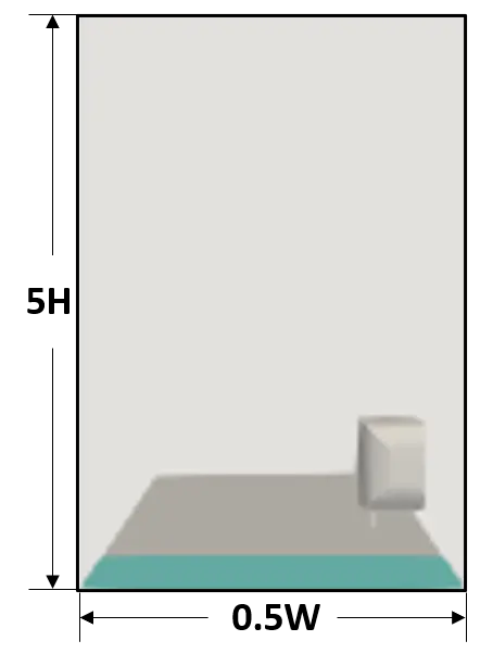
The Ahmed Body as documented by S.R. Ahmed et al., 1984 [1] and the computational domain for simulating air flow movement over it was modelled in SpaceClaim (ANSYS 2021 R1). Dimensions of the computational domain (or virtual wind tunnel) were estimated with respect to the LSTM low speed wind tunnel experiments performed by H. Lienhart et al., 2003 [2] and the recommendations in the ERCOFTAC workshop on Refined Turbulence Modelling [3] which included the length behind the Ahmed Body to be equivalent to five times the bluff body model length and overall width and height as five times the bluff body model width and height values respectively as illustrated in Fig. 2. In regards to the length of the domain from the Inlet boundary to the Ahmed Body along the direction of flow, the region was divided into slip and law of wall boundary surfaces, such that for the latter, a boundary layer thickness of 30mm was attained about 400mm in front of the Ahmed Body, as was specified in the ERCOFTAC test case 9.4 [4], while for the former the length was considered to be almost twice the Ahmed Body model length. This configuration of the computational model ensures a sufficient length for the incoming velocity profile to impose on the bluff body, negligible interaction of the outflow conditions with the bluff body wake and a blockage ratio of nearly 4% (ratio of frontal projected area of the object viz., the bluff body, to the cross-sectional area of the domain surrounding the structure i.e., the wind tunnel, in the direction of flow) which is similar to the experimental setup by H. Lienhart et al., 2003 [2] and was then subsequently imported into Converge Studio v3.0 as a '.stl' file. The basic element entity in CONVERGE is denoted by a triangle which would be visible by clicking on any of the surfaces of the recently drawn model and in order to demarcate boundaries, the corresponding triangles need to be grouped together. The grouping and creation of new boundaries process began with clicking on the 'Boundary' button under the 'Geometry' dock which was followed by clicking on the '+' symbol from which the pop-out message would read as 'Create a new boundary.' leading to the 'Boundary definition' window to open in which the option 'Create multiple boundaries' was checked with number of boundaries as 5, in this case, followed by lastly grouping the triangles that constitute a given surface and naming them accordingly, such as 'Inlet', 'Outlet', 'Slip', 'Ground', 'Symmetry' and an already existing boundary titled 'body' which was renamed to 'Ahmed Body' as illustrated in Fig. 2. Moreover, the normal from each of the triangular surface is required to point towards the fluid domain which was ensured by first visualising the same using the 'Normal toggle' button accessible in the 'View Toolbar' and depending on the direction along which the normal is pointing, a decision was taken by clicking on the 'Normal' tab within the 'Transform' button under the 'Geometry' dock and selecting the suitable option from one of the three 'Transform Normal Options' followed by clicking on the 'Apply' button. At this stage and for the given numerical analysis, the modelling requirements were achieved, however, to validate if the model was clean i.e., it contains no intersecting edges, overlapping triangles or any other form of geometrical constraints, a check was performed by clicking on the 'Find' button in the 'Diagnosis' dock to observe for any anomalous 'Problem Triangles' and rectify the same.
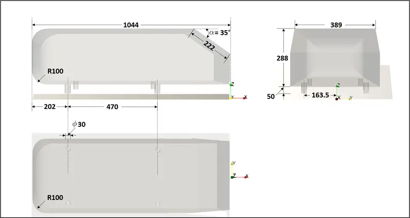
Fig. 1: Measurements superimposed on different three-dimensional viewing planes of the Ahmed Body model (All linear and angular dimension(s) are in mm and degrees respectively)

(a) Front View (b) Side View
Fig. 2: Fluid Volume Model and Boundary Conditions regions (L, H, and W refers to the dimensional attributes of the full-size Ahmed Body)
2.2 Meshing
The meshing approach adopted for the given computational domain was developed to maintain the meshing quality attributes viz., aspect ratio, skewness, and non-orthogonality as outlined in the CONVERGE 3.0 Manual [5] provided in the following table:
|
Aspect Ratio |
1 (Ideal Value) |
||
|
Skewness |
0° (Ideal Value) |
< 70° (Acceptable) |
`>=` 90° (Likely to cause simulation failure) |
|
Non-Orthogonality |
0° (Ideal Value) |
< 70° (Acceptable) |
`>=` 90° (Likely to cause simulation failure) |
Table 1: Mesh Quality Attributes as defined in the CONVERGE 3.0 Manual [5]
The reason for pursuing the above mentioned mesh quality attributes, as specified in Table 1, can be ascertained on the fact that whether the discretized domain was likely to create convergence issues during the solution process and also to identify areas in the mesh where the statistics can be improved based on the underlying physics. In 2.3.3 Determination of Reynolds number from flow velocity and Mesh Refinement approach, detailed discussion about the refined mesh that was prepared and its mesh qualities has been highlighted.
2.3 CFD Simulation Setup, Boundary Conditions, Monitoring Variables, Determination of flow velocity from given Reynolds number and Solution
The simulation on a single mesh configuration for the computational domain based on the Ahmed Body model having a slant angle of 35° was performed using the Reynolds Averaged Navier-Stokes (RANS) models, in this case, the k-`epsilon` turbulence models. The use of k-`epsilon` turbulence models, more specifically the RKE turbulence models, is attributed to the fact that the Reynolds number, based on the given flow conditions, lies in the turbulence flow region and that it is capable of predicting the physics involved for fluid flows exhibiting boundary layer separation and boundary layers under the influence of strong adverse pressure gradients for which the solution variables, like the velocity profile, was modelled for the log-law layer using the standard wall function approach such that the first grid cell would lie in the range of 30<`y^+`<300 in order to yield satisfactory results. A brief description into the working of the RKE turbulence model is provided below:
2.3.1 RKE turbulence model
The RKE turbulence model proposed by Shih et al., 1995 [6] is considered as an upgrade to the standard k-`epsilon` turbulence model while sharing the similarities of consisting two transport equations, one for the turbulent kinetic energy (k) to evaluate the energy in turbulence and the other for the turbulent dissipation (`epsilon`) to calculate the rate of dissipation of turbulent kinetic energy (k), however notable differences are present as mentioned below:
- The turbulent viscosity term is formulated differently in the RKE turbulence model.
- The dissipation rate `epsilon` in the transport equation has been modified and developed from the exact equation for transport of mean-square vorticity fluctuation.
The RKE turbulence model is able to satisfy some of the mathematical constraints of the Reynolds's stresses such as the positive values of normal stresses when the eddy viscosity definition is used in the Boussinesq relationship and Schwarz inequality for shear stresses even when the main strain rate is large which otherwise would be negative. These formulations in the RKE turbulence model have made them more popular to use over the other k-`epsilon` turbulence models especially when flow features include the presence of strong streamline curvature, vortices, rotation, boundary layers under the influence of strong and adverse pressure gradients, separation and recirculation.
2.3.1.1 Setup of the RKE turbulence model:
To use the RKE turbulence model in Converge Studio v3.0, we navigate to Physical Models option in the Case Setup tree followed by checking the 'Turbulence modeling' box to enable inclusion of turbulence terms in the solution of governing fluid equations and then selecting the Reynolds Averaged Navier-Stokes (RANS) item in the 'Turbulence modeling' window available under the Physical Models option with 'Turbulence model' drop-down menu set to 'Realizable k-`epsilon`' and 'Near Wall treatment' retained at its default selection of 'Standard wall function' while all other variables/parameters and constants remained unaltered with respect to their original values.
2.3.2 Boundary Conditions and Monitoring Variables
The different boundary conditions for the computational domain based on the Ahmed Body model having a slant angle of 35° is described in the following table:
|
Names |
Inlet |
FreeSlip |
Ground |
Symmetry |
AhmedBody |
Outlet |
|
Type |
INFLOW |
WALL |
WALL |
-- |
WALL |
OUTFLOW |
|
Pressure Boundary Condition |
Zero normal gradient (NE) |
-- |
-- |
-- |
-- |
Specified Value (DI) |
|
Pressure Magnitude (Pa) |
-- |
-- |
-- |
-- |
-- |
101325 |
|
Velocity Boundary Condition |
Specified Value (DI) |
-- |
-- |
-- |
-- |
Zero normal gradient (NE) |
|
Velocity Magnitude (m/s) |
(u v w) `-=` (40 0 0) [2] |
-- |
-- |
-- |
-- |
-- |
|
Temperature Boundary Condition |
Specified Value (DI) |
Zero normal gradient (NE) |
Zero normal gradient (NE) |
-- |
Zero normal gradient (NE) |
-- |
|
Temperature Backflow |
-- |
-- | -- | -- |
-- |
Specified Value (DI) |
|
Temperature Magnitude (K) |
300 |
-- |
-- |
-- |
-- |
300 |
|
Species Boundary Condition |
Specified Value (DI) |
-- |
-- |
-- |
-- |
Specified Value (DI) |
|
Species Name: `O_2` |
0.23 |
-- |
-- |
-- |
-- |
0.23 |
|
Species Name: `N_2` |
0.77 |
-- |
-- |
-- |
-- |
0.77 |
|
Wall motion type |
-- |
Stationary |
Stationary | -- |
Stationary |
-- |
|
Surface Movement |
-- |
Fixed, Slip |
Fixed, Law of wall | -- |
Fixed, Law of wall |
-- |
|
Turbulent Kinetic Energy (tke) |
Intensity, 0.0025 fraction [2] |
Specified Value (DI) |
Zero normal gradient (NE) |
-- |
Zero normal gradient (NE) |
-- |
|
Turbulent Dissipation (eps) |
Length scale, 0.00807922m |
Zero normal gradient (NE) |
Wall model | -- |
Wall model |
-- |
|
Turbulent Kinetic Energy (tke) Backflow |
-- |
-- | -- | -- | -- |
Intensity, 0.0025 fraction [2] |
|
Turbulent Dissipation (eps) Backflow |
-- |
-- | -- | -- | -- |
Length scale, 0.00807922m |
|
Near wall treatment |
-- |
Global | Standard wall function | -- |
Standard wall function |
-- |
|
Law of wall roughness parameters; Absolute roughness |
-- |
-- | 0.0m | -- | 0.0m | -- |
|
Law of wall roughness parameters; Roughness constant |
-- |
-- | 0.5 | -- | 0.5 | -- |
Table 2: Boundary Conditions for the computational domain based on the Ahmed Body model having a slant angle of 35° defined using the 'Boundary' sub-option of the 'Boundary Conditions' under the 'Case Setup' tree
For the given problem, the simulation was chosen as 'Gas simulation' enabled in the 'Materials' option in the 'Case Setup' tree with 'Predefined mixtures' set to 'Air' and 'Species (not in mech.dat)' option enabled to utilise the mass fraction values of `O_2` and `N_2` as they represent the major constituting species in air by mass fraction. Since, 'Gas simulation' option was checked in the 'Materials' option, an equation of state was required to be defined that formulates a coupling relationship between the different state variables such as density and physical conditions such as pressure and temperature to depict the state of matter. In the given numerical analysis, the Redlich-Kwong (RK) cubic equation of state was set to in the 'Equation of state' drop-down menu with its default values of critical temperature (`T_c`) and critical pressure (`p_c`) retained at '133.0 K' and '3770000.0 Pa' respectively as it is a simpler form of representation in comparison to the Redlich-Kwong-Soave and Peng-Robinson set of equations but more accurate than the ideal gas law which works best for gases at low pressures, however, at higher pressures tends to report huge deviations in its predictions as it assumes that the molecular volume is very small and that neither attraction or repulsion exists between the molecules which is not true in the case of real gases. Additionally, the real gas properties would behave as a function of temperature which was again set to as the default option in the 'Gas simulation' window. The values of 'Turbulent Prandtl number' and 'Turbulent Schmidt number' were left unchanged at their default values of 0.9 and 0.78 respectively.
In regards to specifying the turbulence length scale, it was decided to choose a value of 0.4 times the boundary layer thickness as part of an external flow simulation setup. Additionally, the 'Boundaries only' option was selected under the 'Wall Output' list of the 'Output files' sub-option of the 'Output/Post-Processing' item under the 'Case Setup' tree to visualise the drag and lift forces acting on the Ahmed Body during the solution process.
2.3.3 Determination of Reynolds number from flow velocity and Mesh Refinement approach
Reynolds number (based on Ahmed Body model length):
`Re = (U*L*rho)/mu`; where (Eq. 1)
`U` is the freestream velocity,
`L` is the characteristic length, in this case, the Ahmed Body model length,
`rho` is density of fluid, and
`mu` is the dynamic viscosity of fluid
Substituting the value of characteristic length as Ahmed Body model length of 1.044m, and density and dynamic viscosity of air at 1atm or 101235 Pa and 300K (or 26.85°C) as 1.1766 `(kg)/(m^3)` and `1.857*10^-5 (kg)/(m.s)` [7] respectively into (Eq. 1), a corresponding Reynolds number of 2645924.39 was estimated for flow velocity of 40m/s [2]. Boundary layer thickness, in case of turbulent flow, is usually dependent on experiments and/or empirical relations as it difficult to predict the same because of the intense mixing of different layers involved within it. Since, the value of Reynolds number determined suggests that it exceeds the engineering critical Reynolds number of `5*10^(5)` and is in the transitional regime being relatively closer to the peak point of the transition Reynolds number of `3*10^(6)` beyond which the boundary layer is deemed to be fully turbulent with respect to smooth flat plate geometrical considerations under uniform upstream conditions, it was decided to evaluate the boundary layer thickness based on turbulent flow conditions which was determined using the mathematical expression shown below:
`(delta/x) = 0.16/(Re_x)^(1/7)`; where (Eq. 2)
`delta` is the boundary layer thickness, and
`Re_x` is the Reynolds number for the characteristic length i.e., length of the bluff body (L)
For the given Reynolds number and Ahmed Body model length, the turbulent boundary layer thickness using Eq. 2 is determined to be 0.020198049m. To perform calculations for `y^+` value, the values of wall shear stress and frictional velocity were required to be calculated as shown below:
Wall Shear Stress:
`tau_w=(1/2)⋅C_f⋅rho⋅(U_∞)^2`; where (Eq. 3)
`tau_w` is Wall shear stress,
`C_f` is Skin Friction coefficient,
`U_∞` is the freestream velocity, in this case the calculated value of inlet boundary velocity
Skin Friction Coefficient (`C_f`) based on a semi-empirical expression can be related to the Reynolds number as shown below:
`C_f = 0.027/(Re_x)^(1/7)`, where (Eq. 4)
Frictional velocity (`U_tau`) can be computed mathematically as:
`U_tau=sqrt(tau_w/rho)` (Eq. 5)
For local Reynolds number of 2645924.39 with the previously mentioned values of dynamic viscosity, density and free-stream velocity, the skin-friction coefficient (`C_f`), wall shear stress (`tau_w`) and friction velocity (`U_tau`) values were calculated using (Eq. 4), (Eq. 3) and (Eq. 5) respectively as shown in the following table:
|
Local Reynolds Number |
Skin-friction Coefficient (`C_f`) |
Wall Shear Stress (`tau_w`)[kg m^-1 s^-2] |
Friction Velocity (`U_tau`)[m s^-1] |
|
2645924.39 |
`3.265*10^(-3)` |
3.0731 |
1.6161 |
Table 3: Skin-friction coefficient, wall shear stress and friction velocity values for the governing flow conditions of the computational domain based on the Ahmed Body model having a slant angle of 35°
(Eq. 2) was also reutilised to determine the length at which the boundary layer thickness attains a value of 30mm, 400mm in front of the Ahmed Body, based on the value of Reynolds number achieved considering the Ahmed Body model length resulting into a value of 1.656m approximately and was taken into consideration during the modelling of the computational domain as was mentioned in Section 2.1 Modelling.
Calculation of cell-centroid size (`y_P`), First Cell Height (`Delta_y`) and embed scale with respect to Base Grid Size:
`y^+` is defined as the non-dimensional wall distance for a wall bounded flow that can be expressed mathematically as:
`y^+=(ρ*U_tau*y_P)/mu`; where (Eq. 6)
`y_P` is distance from the cell-centroid 'P' to the wall
Simplifying (Eq. 6) to determine `y_P`, we get;
`y_P=(y^+*mu)/(U_tau*rho)` (Eq. 7)
Since, `y^+` is computed at the cell-centroid, the first cell height (`Delta_y`) can accordingly be mathematically expressed as:
`Delta_y = 2*y_P` (Eq. 8)
The initial approach adopted for evaluating the distance from the cell-centroid 'P' to the wall (`y_P`) and correspondingly the first cell height (`Delta_y`) was to target a `y^+` value such that the first grid cell would lie in the range of 30<`y^+`<300 for the RKE turbulence model so as to implement the wall modelling strategy for the log-law layer using the standard wall function approach. However, due to constraints in computational resources, including limitations in number of mesh cells to 500000, and only 4 cores available on the author's PC, a single transient simulation was estimated to take upwards of 4 hours of actual run time, derived from a single run for a coarse mesh, and therefore, it was decided to prepare only a single mesh wherein the empirically estimated `y^+` value on the Ahmed Body was under 300.
From the CONVERGE 3.0 Manual [5], the mathematical formulation relating the embed size with the base grid size based on embed scale can be given by:
`embed = (base grid)/(2^(EMBED SCALE))`; where (Eq. 9)
`base grid` is the Base Grid Size defined for every element across the domain,
`EMBED SCALE` is the scaling parameter by which the base grid size is to be refined either at the selected boundary, geometrical shape or region, and
`embed` is the scaled down or refined grid size, in this case also equal to the First Cell Height i.e., `Delta_y`,
The missing variable in (Eq. 9) is `EMBED SCALE` and therefore equating for the same variable was required with regards to the given grid size.
|
Mesh |
dx(m) |
dy(m) |
dz(m) |
|
1 |
0.08 |
0.08 |
0.08 |
Table 4: Mesh size representing spatial grid discretization values across each of the three-directional axes
|
Mesh |
Entity Type |
`EMBED SCALE` |
Embed Layers |
Target First Cell Height (`Delta_y`)[m] |
Target `y^+` (`y_P`) |
Size of Refinement Region |
|
1 |
Boundary |
4 |
5 |
0.005 |
~260 |
-- |
|
1 |
Box |
1 |
-- |
0.04 |
-- |
3L*0.625W*H |
Table 5: `EMBED SCALE`, Embed Layers, Target First Cell Height (`Delta_y`), Target `y^+`(`y_P`) and Size of Refinement Region for the Box Entity Type Fixed Embedding with regards to mesh 1 configuration of the computational domain based on the Ahmed Body model having a slant angle of 35° (L, W and H refer to the dimensions of the full size Ahmed Body to scale)
It should be noted that the values of `EMBED SCALE` and Embed Layers were required to be positive integers which was duly considered before arriving at the above mentioned specifications.
Mesh 1:

Fig. 3: Mesh 1 (two-dimensional sliced view)
2.3.4 Determination of transient parameters for the fluid flow material across the computational domain
The setup of simulation run time and time-step for the given numerical problem with respect to the fluid material was defined such that the 'Start time' in the 'Simulation Time parameters' window under the 'Case Setup' tree was set to 0s while the 'End Time' in the same window depended on the domain length and the flow velocity, in the direction of flow, such that the fluid medium passed through it at least 10 flow through times so as to achieve steady state conditions or observe a consistent transient behaviour. Therefore, 'End Time' was evaluated as:
`End Time = (L/U)*10`; where (Eq. 10)
`L` is the length of the computational domain in the direction of flow determined as 10.4083m
From (Eq. 10), the value of 'End Time' obtained is approximately equal to 2.6021s. Time-step was decided based on the CFL number which is expressed below:
`CFL = (U*Delta t)/(Delta x)`; where (Eq. 11)
`Delta t` is time-step,
`Delta x` represents the smallest cell size, which in this case was the value of the First Cell Height in the turbulent boundary layer thickness on the Ahmed Body
In order to attain temporal accuracy and numerical stability, the CFL criteria was decided to be 1 and therefore, the value of time-step determined with this limiting value for different mesh sizes have been reported in Table 6.
| Mesh | `Delta t` (s) |
| 1 | 0.000125 |
Table 6: Time-step (`Delta t`) values for mesh 1 configuration of the computational domain based on the Ahmed Body model having a slant angle of 35°
The above value of time-steps reflect for a domain whose smallest cell size across it would remain at the value of `Delta x`, as reported earlier, however, with the cartesian cut-cell meshing approach, the same cannot always be achieved and therefore, the time marching solution process or 'Time-step selection' chosen was of type 'Use variable time-step algorithm'. A variable time-step allows for internally calculated time-step that in turn depends on additional inputs including minimum and maximum time-step, and maximum convection CFL, among others, such that the resultant value determined based on the corresponding limiting conditions on the inputs would represent the maximum permissible time-step for the next iteration to be performed. The initial, minimum and maximum time-step chosen for each setup is tabulated as seen in Table 7 below wherein the initial and minimum time-step were chosen to be a value that would be a reasonably good start for the simulation, considering the given setup, while the maximum time-step represents the `Delta t` values as calculated in Table 6.
| Mesh | Initial time-step (s) | Minimum time-step (s) | Maximum time-step (s) |
| 1 | 1e-9 | 1e-9 | 0.000125 |
Table 7: Initial, minimum and maximum time-step values for mesh 1 configuration of the computational domain based on the Ahmed Body model having a slant angle of 35°
Mesh and time statistics, average and minimum `y^+` values, and pressure drag force values on the Ahmed Body for mesh 1 configuration:
|
Mesh |
Cells |
Run Time [s] |
Average `y^+` on Ahmed Body |
Minimum `y^+` on Ahmed Body |
Pressure Force (Drag) [N] on Ahmed Body |
|
1 |
270034 |
58270.249 |
200.451 |
51.2039 | 33.5314 |
Table 8: Mesh and time statistics, average and minimum `y^+` values, and pressure drag force values on the Ahmed Body for mesh 1 configuration
Mesh quality attributes for mesh 1 configuration of the computational domain based on the Ahmed Body model having a slant angle of 35°:
|
Mesh |
Max Aspect Ratio |
Max Skewness |
Max Non-Orthogonality |
|
1 |
3.36438 |
1.17578e-38 |
65.7723 |
Table 9: Mesh quality attributes depicting the maximum values of aspect ratio, skewness and non-orthogonality for mesh 1 configuration of the computational domain based on the Ahmed Body model having a slant angle of 35°
Coefficient of drag (`C_D`) is a dimensionless quantity and can be defined as the ratio of the pressure drag force (major component of the net drag force as a result of the influence of the shape of the bluff body), `F_D`, acting on the Ahmed Body to the force produced by the dynamic pressure times the area that is expressed mathematically below as:
`C_D=F_D/(0.5*ρ*U^2*A)`; where (Eq. 12)
`A` refers to the frontal area or the area projected onto a plane normal to the direction of flow, in this case equal to 0.112`m^2` with respect to the full-size Ahmed Body
From Table 7, it can be seen that the prediction of drag force on the Ahmed Body using the RKE turbulence model for the above specified mesh 1 configuration leads to a drag coefficient value of 0.3181 from (Eq. 12) which in comparison to experimental findings of 0.2790 by Meile et al., 2011 [8] and 0.2580 by S.R. Ahmed et al., 1984 [1] for the same Ahmed Body model having a slant angle of 35° reports a deviation of about 14.014% and 23.294% respectively clearly implying the need for further mesh refinement. It can also be observed that the minimum `y^+` value estimated for the same mesh configuration lies in the log-law layer justifying the use of standard wall function as the near wall treatment modeling approach for the RKE turbulence model with respect to the given problem. Additionally, mesh quality attributes of the same mesh configuration prepared in Table 9 indicates that they lie in the range of acceptable value for skewness and non-orthogonality, as previously stated in Table 1, with the aspect ratio deviating from an ideal value of 1, especially close to the Ahmed Body.
2.4 Post-Processing
The extended part of the solution process using Converge Studio v3.0 included selecting the variables of interest whose quantitative and qualitative aspects would highlight the behaviour of the flow, in this case within the given fluid domain and over the Ahmed Body model, and they can be chosen by clicking on the 'Post variable selection' sub-option of the 'Output/Post-Processing' setting under the 'Case Setup' tree and checking the boxes 'Density', 'Mesh Quality', 'Pressure', 'Temperature', 'Velocity' and 'Vorticity 'in the 'Typical Variables' section and 'Region ID' in the 'Geometry/Location' section of the 'Typical Variables/Geometry' tab, 'Turbulent Kinetic Energy', 'Turbulent Length Scale', 'Turbulent Viscosity', 'Dissipation Rate of tke (eps)', and '`y^+`' in the 'Turbulence' section of the 'Combustion/Turbulence' tab, and adding 'Mass Fraction' under 'Species' section of the 'Species/Passive' tab for `O_2` and `N_2` species with respect to the concerned numerical analysis. Visualising the different flow variable quantities in a two-dimensional space in ParaView required the creation of a slice of the given fluid domain by using the "Slice" tool in the 'Commons' toolbar typically located above the 'Pipeline Browser' window based on default layout settings and choosing 'Y Normal' and 'X Normal' under 'Plane Parameters' section to align the plane normal such that the entire domain was viewed in the direction of flow and perpendicular to the y-axis direction to observe the wake regions respectively followed by unchecking the 'Show Plane' and 'Triangulate the slice' boxes for disabling the viewing of the plane borders and production of triangles in the output respectively. Plotting the velocity (x-component) profiles for the validation case was performed by using ParaView's in-built "plot over line" tool. The "plot over line" tool was accessed by clicking on 'Filters' present in the data analysis group, followed by entering the coordinates as seen from Table 10 to Table 17 before clicking on the "Apply" button to view the said profiles.
|
Line 1 |
x |
y |
z |
|
Point 1 |
-0.013 |
0 |
0.236 |
|
Point 2 |
-0.013 |
0 |
0.738 |
Table 10: Line Coordinates for viewing the velocity (x-component) profile at x=-0.013m with respect to the origin of the given domain
|
Line 1 |
x |
y |
z |
|
Point 1 |
-0.063 |
0 |
0.271 |
|
Point 2 |
-0.063 |
0 |
0.738 |
Table 11: Line Coordinates for viewing the velocity (x-component) profile at x=-0.063m with respect to the origin of the given domain
|
Line 1 |
x |
y |
z |
|
Point 1 |
-0.113 |
0 |
0.306 |
|
Point 2 |
-0.113 |
0 |
0.738 |
Table 12: Line Coordinates for viewing the velocity (x-component) profile at x=-0.113m with respect to the origin of the given domain
|
Line 1 |
x |
y |
z |
|
Point 1 |
-0.263 |
0 |
0.363 |
|
Point 2 |
-0.263 |
0 |
0.738 |
Table 13: Line Coordinates for viewing the velocity (x-component) profile at x=-0.263m with respect to the origin of the given domain
|
Line 1 |
x |
y |
z |
|
Point 1 |
0.037 |
0 |
0.028 |
|
Point 2 |
0.037 |
0 |
0.738 |
Table 14: Line Coordinates for viewing the velocity (x-component) profile at x=0.037m with respect to the origin of the given domain
|
Line 1 |
x |
y |
z |
|
Point 1 |
0.087 |
0 |
0.028 |
|
Point 2 |
0.087 |
0 |
0.738 |
Table 15: Line Coordinates for viewing the velocity (x-component) profile at x=0.087m with respect to the origin of the given domain
|
Line 1 |
x |
y |
z |
|
Point 1 |
0.137 |
0 |
0.028 |
|
Point 2 |
0.137 |
0 |
0.738 |
Table 16: Line Coordinates for viewing the velocity (x-component) profile at x=0.137m with respect to the origin of the given domain
|
Line 1 |
x |
y |
z |
|
Point 1 |
0.187 |
0 |
0.028 |
|
Point 2 |
0.187 |
0 |
0.738 |
Table 17: Line Coordinates for viewing the velocity (x-component) profile at x=0.187m with respect to the origin of the given domain
It was ensured that the last time-step size of the simulation run was selected to view the velocity (x-component) profile results. Additionally, pressure (p) field plots were created to view the development of the flow field characteristics across the fluid domain and on the Ahmed Body while Stream Tracer was added for identifying the separation and recirculation regions around the bluff body. Legends, titles, and x and y labels were added for better understanding of the graphical representations. To save an animation file of the different field plots, the option 'Save Animation' was accessed under the 'File' menu and clicked on followed by choosing the appropriate settings under the different sections such as 'Size and Scaling', 'Coloring', 'Compression Options' and 'Animation Options' to name a few, assigning an appropriate name to the animation file, in this case by the variable whose field plot is being indicated before clicking on the 'OK' button.
2.5 Convergence Level
In the given computational analysis, a transient simulation using first-order implicit Euler time advancement scheme was performed to accommodate for larger time-steps while also being numerically stable along with a Density-based solver of type modified Pressure Implicit with Splitting of Operator (PISO) which is an iterative pressure-velocity coupling algorithm involving a predictor step for predicting solution of the momentum equation from which a pressure equation is obtained and solved whose correction is then consequently reapplied to the momentum equation such that this process continues until the desired level of accuracy is achieved. At the end of the momentum predictor and first corrector step, remaining transport equations are solved in series. In other words, momentum and pressure are solved at the first PISO iteration which enables calculation for velocity terms required by other transport equations and at the end of each iteration in the PISO loop, convergence criterion is checked for which in this case requires the density correction error term to be less than the value of PISO tolerance which remains unchanged for the given numerical simulation at its default value of 1e-03. The selection of solver types for the different equations within 'Solver parameters [Transient]' sub-option in the 'Simulation Parameters' settings under the 'Case Setup' tree included assigning SOR to Momentum, Pressure, Density, Energy, Turbulent Kinetic Energy (tke) and Turbulent dissipation rate (eps) equations. The SOR solver type is a generally preferred algorithm owing to its advantage in being computationally less expensive than the different forms of biconjugate gradient stabilized (BiCGSTAB) algorithms or HYBRID (wherever applicable). The solver types, convergence tolerance limits, and minimum and maximum iterations defined for the equations corresponding to the RKE turbulence model equations for the transient state simulation and the monitor variable plots corresponding to the behaviour of pressure force (drag) on the surface of the Ahmed Body are shown in the table and figure below:
|
Equations |
Solver Type |
Convergence Tolerance |
Minimum Iterations |
Maximum Iterations |
Preconditioner |
|
Momentum |
SOR |
1e-05 |
2 |
50 |
None |
|
Pressure |
CONVERGE BiCGSTAB |
1e-08 |
2 |
500 |
None |
|
Density |
SOR |
1e-04 |
2 |
20 |
None |
|
Energy |
SOR |
1e-04 |
2 |
20 |
None |
|
Turbulent Kinetic Energy (tke) |
SOR (pre-defined) |
1e-03 |
2 |
50 |
None (pre-defined) |
|
Turbulent dissipation rate (eps) |
SOR (pre-defined) | 1e-03 | 2 | 50 | None (pre-defined) |
Table 18: Solver Types, Convergence Tolerance Values, Minimum and Maximum Iterations and Preconditioners of the different equations used in the RKE turbulence model
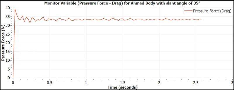
Fig. 4: Pressure force (drag) boundary variable plot with respect to transient simulation on the Ahmed Body having a slant angle of 35° using RKE turbulence model for mesh 1
From Fig. 4, we can notice that the monitor variable shows a cyclic output with almost similar trends in terms of variations whose intensity gradually continues to decrease over the given time period specified in the 'End time' parameter under the 'General' tab of 'Simulation Parameters' settings under the 'Case Setup' tree as 2.6021s indicating that the solution has nearly arrived at steady-state conditions.
3. Results
3.1 Validation of normalised velocity (x-component) values against experimental data using line plots
Fig. 5 below shows the comparison of the normalised streamwise velocity component profiles towards and along the rear part of the Ahmed body for slant angle of 35° wherein it can be noticed that the numerically simulated results shows reasonable agreement against the experimental data at different x locations as was specified in Section 2.4 Post-Processing. There are, however, noticeable disagreements especially close to the slant surface as the flow separation begins to take place and subsequently downstream as the wake region enlarges indicating that the gradients require more or better quality cells to capture the physics of the flow in and around the region. It should be noted that an amplification factor of 10 was considered to enhance the visualisation of the said profiles.
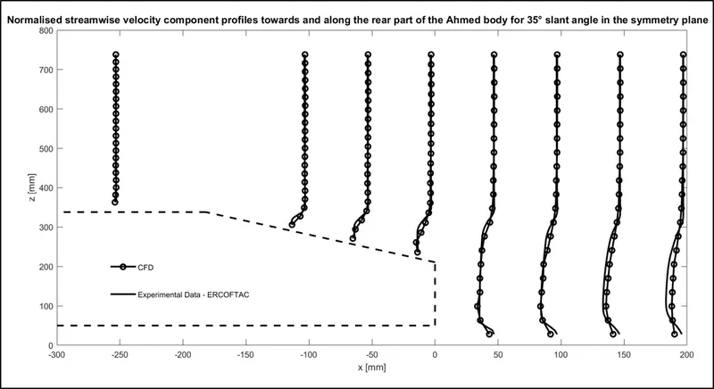
Fig. 5: Normalised streamwise velocity component profiles towards and along the rear part of the Ahmed body for 35° slant angle in the symmetry plane
3.2 Wake region behind the Ahmed Body using velocity and static pressure field plots
Fig. 6 shows the velocity field plot at the slice region created by orienting the plane normal to the flow direction as was specified in Section 2.4 Post-Processing with the Ahmed Body coloured using pressure values at different time step numbers while Fig. 7 highlights the intensity of the wake region at two different streamwise slice planes coloured by vorticity magnitude for mesh 1 configuration. It can be noticed that the velocity impinging on the fore body region comes to a complete standstill creating a zone of high pressure immediately in front of it before getting deflected. As the flow progresses from the fore body to the mid-section and from the mid-section to the slant, a massive pressure drop is experienced by the flow, as a result of changes in the geometry, before leaving the vehicle body at the rear end as the velocity begins to accelerate in order for the fluid flowing across the bluff body to adhere to its surface. Across the slant surface and for the given configuration of the Ahmed Body, the fluid flow separates yet again for the same reasons of geometrical construction as mentioned previously, leading to a lowering of pressure levels which because of the vortex mechanism involved causes the creation of a recirculatory region indicating the presence of a wake region beyond the bluff body. The intensity of wake is stronger near the rear end of the bluff body before eventually weakening further away from it in the direction of flow.
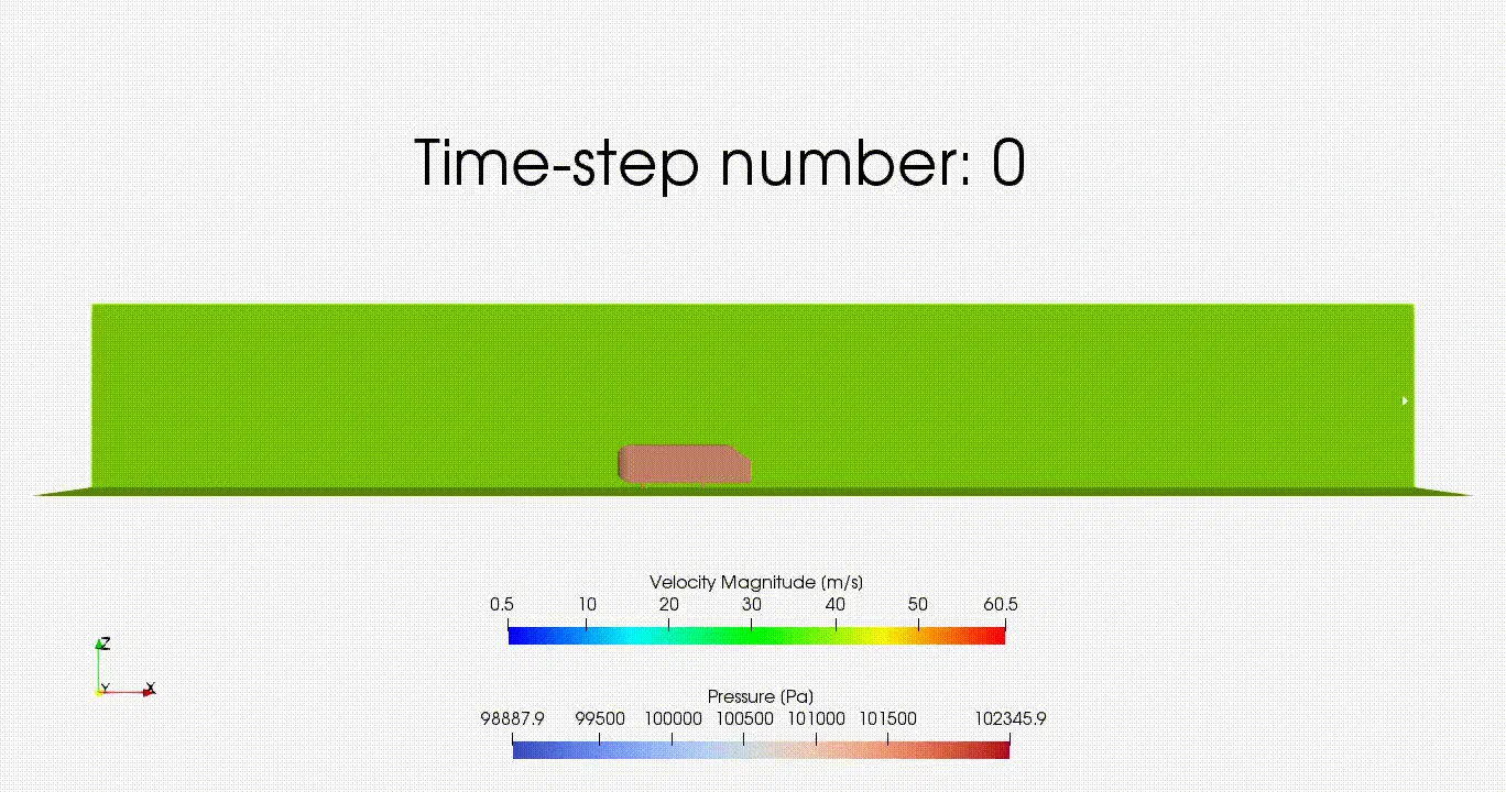
Fig. 6: Animation of the velocity field plot at the slice region created by orienting the plane normal to the flow direction with the Ahmed Body coloured using pressure values at different time step numbers
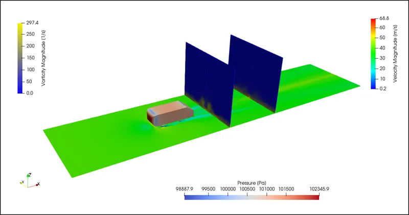
Fig. 7: Velocity field plot on the 'Ground' boundary surface with the Ahmed Body coloured using pressure values and two different planes in the direction of flow coloured using vorticity magnitude
4. Discussion
Air, containing a mixture of two major contributing gas species `O_2` and `N_2` by mass fraction, enters at the inlet of the given cross-section of the computational domain consisting of a bluff body, in this case the Ahmed Body, as a turbulent flow which deflects away at the forebody region due to its rounded surface causing decrease in the velocity with subsequent increase in pressure. The flow continues along the surface as a result of its continuous motion before encountering another sudden change in geometry closer to the onset of the mid-section leading to separation followed by low pressure values before the fluid accelerates to reattach itself to the bluff body. This behaviour of flow separation and reattachment leads to generation of longitudinal vortices further downstream and along the mid-section of the body which is an attribute of the attached turbulent boundary layer. As the flow nears the slant edge, the flow phenomena becomes increasingly complex with strong dependence on the value of the slant angle such that for the given configuration, the flow detaches near the top of the given surface forming a single large wake region behind the bluff body, identified with reverse flow or as a low-pressure region, with the almost fuller turbulent profile going on to form a reattachment point further downstream, depending on the length of the domain.
5. Conclusion
The three-dimensional and transient numerical analysis of the Ahmed Body using RKE turbulence model in Converge Studio v3.0 and executed using the Cygwin64 terminal was well understood. It was realised that using an appropriate wall modelling approach like the standard wall function with respect to the empirically estimated `y^+` values, the numerical simulation was able to reproduce the flow characteristics around the bluff body to a reasonable agreement and also the drag coefficient predicted being in a similar range as those determined experimentally albeit with the limitations on computational resources and meshing constraints. An improved mesh or different meshing approach that would capture the gradients better especially in the flow separation area at the rear end is required to be investigated and is under consideration from a future scope of study.
References
[1] S.R. Ahmed, G. Ramm, Some Salient Features of the Time-Averaged Ground Vehicle Wake, SAE-Paper 840300, 1984
[2] H. Lienhart, C. Stoots, S. Becker, Flow and Turbulence Structures in the Wake of a Simplified Car Model (Ahmed Model), DGLR Fach Symp. der AG STAB, Universität Stuttgart, November 15–17, 2003
[3] R. Manceau, J.Bonnet, eds., 10th joint ERCOFTAC/IAHR/QNET-CFD Workshop on Refined Turbulence Modelling, Poitiers, France 2002
[4] ERCOFTAC - European Research Community on Flow, Turbulence and Combustion (2001, 2002)
[5] CONVERGE 3.0 Manual. © 2020 Convergent Science. All rights reserved. July 15, 2020.
[6] Shih, T.-H., Liou, W.W., Shabbir, A., Yang, Z., and Zhu, J., "A New k-ε Eddy Viscosity Model for High Reynolds Number Turbulent Flows—Model Development and Validation," Computers & Fluids, 24(3), 227-238, 1995. DOI: 10.1016/0045-7930(94)00032-T
[7] Engineers Edge, LLC, Viscosity of air, Dynamic and Kinematic, www.engineersedge.com, viewed 26 August 2021, <https://www.engineersedge.com/physics/viscosity_of_air_dynamic_and_kinematic_14483.htm#:~:text=The%20viscosity%20of%20air%20depends,2%20%2Fs%20or%2014.8%20cSt.>
[8] W. Meile, G. Brenn, A. Reppenhagen, B. Lechner, A. Fuchs, Experiments and numerical simulations on the aerodynamics of the Ahmed body, CFD Letters, Vol. 3 (1) – March 2011