Week 3: Flow over a backward facing step

1. Introduction

Turbulent fluid flow can be described as motion of fluid characterised by irregular and erratic changes in field quantities such as pressure and velocity due to the build-up of excessive kinetic energy leading to mixing between fluid layers and subsequently increasing frictional drag within the medium. Typically, most fluid flows existing in nature and in many engineering applications tend to be turbulent and more often than not the surfaces over which they travel never always remains consistently uniform in terms of the contour leading to the possibility of separation and reattachment along its direction of travel.

The aim of this challenge was to perform two-dimensional, steady-state simulations, using Realizable k-`epsilon` (RKE) turbulence model for a backward-facing step (BFS) geometry. The analysis involved computing results for different grid sizes that would outline total cell count, velocity magnitude profiles, pressure drop values across the domain, mesh verification and validation against analytical formulations, identification of separation and recirculation region as well as mesh quality attributes like skewness, non-orthogonality, and aspect ratio.

2. Method

The typical approach adopted to performing numerical simulations in CONVERGE CFD involves the following steps:

1. Creating a new folder dedicated to running the concerned project inside a user-preferred directory.
2. Setting up the relevant case file(s) in Converge Studio v3.0 that involves creation of the fluid volume domain, setting up the required application type, choosing material and its state (gas, liquid, parcel or solid) for which simulation is to be performed along with the requisite properties, defining simulation parameters such as solver types, monitor variables, run time variables, and convergence tolerances, defining region(s), boundary conditions and initial conditions, specifying the physical models whose equations are intended to be solved, determining and allocating the base grid size values and lastly selecting the variables for post-processing at the required time intervals (in terms of cycles for steady-state) along with any hidden parameters or UDF selection as part of advanced parameters.
3. Saving the case file(s) and exporting the input files into the folder created for running the concerned project which typically includes 'boundary.in', 'material_state.dat' where material_state points to either 'gas', 'liquid', 'parcel' or 'solid', 'initialize.in', 'inputs.in', 'monitor_steady_state.in', 'post.in', 'solver.in' and 'surface.dat' while other input files with respect to the state of the material, thermal properties and species may also be part of the exporting process and should be ensured that they are selected for the simulation to run.
4. Running the simulation in a Cygwin64 terminal window.
5. Post-converting 3D output data by navigating to the output folder created within the same project folder during the simulation run or from the 'Post-Processing 3D' button in Converge Studio v3.0.

The simulation run and post-converting processes were executed using Linux-type commands in a Cygwin64 terminal window as shown below:

i) Change directory to the project containing the relevant case file(s):

cd "PATH_TO_CONCERNED_PROJECT_FOLDER"

ii) Confirm the contents of the project for the exported input files:

ls

iii) Performing simulation run with the converge executable application on multiple processors (in this case, 4) using mpiexec executable file in the background (by adding ampersand operator) along with posting output into a logfile:

mpiexec.exe -n 4 converge.exe restricted </dev/null> logfile &

iv) Checking for simulation status with regards to completion or errors:

tail logfile

v) Post-converting the 3D output data files using the 'post_convert_30_msmpi_64' utility on multiple processors (in this case, 4) using mpiexec executable file from within the output folder of the project containing the exported input files:

cd output

mpiexec.exe -n 4 post_convert_30_msmpi_64

2.1 Modelling

The BFS computational domain for simulating air flow movement through it was modelled in Converge Studio v3.0. The length of the domain along z-axis, or the width, was considered to be sufficiently long such that the variations in field quantities were almost negligible in that direction, similar to the experimental analysis conducted by Driver and Seegmiller [1], thereby allowing the assumption of carrying out simulations in a two-dimensional setup to be valid by selecting the appropriate boundary types on the different boundary zones. The extents of the BFS model were provided as 0.272009m in the direction of flow (or x-axis), and 0.00855m and 0.0199757m as the inlet and outlet diameters respectively at either ends of the length of the domain along the y axis. The basic element entity in CONVERGE is denoted by a triangle which would be visible by clicking on any of the surfaces of the recently drawn model and in order to demarcate boundaries, the corresponding triangles needed to be grouped together. The grouping and creation of new boundaries process began with clicking on the 'Boundary' button under the 'Geometry' dock which was followed by clicking on the '+' symbol from which the pop-out message would read as 'Create a new boundary.' leading to the 'Boundary definition' window to open in which the option 'Create multiple boundaries' was checked with number of boundaries as 5, in this case, followed by lastly grouping the triangles that constitute a given surface and naming them accordingly, such as 'Inlet', 'Outlet', 'Top Wall' and 'Bottom Wall' (together named as 'TopBottomWalls'), 'Front2D' and 'Back2D' as illustrated in Fig. 1. Moreover, the normal from each of the triangular surface is required to point towards the fluid domain which can be ensured by first visualising the same using the 'Normal toggle' button accessible in the 'View Toolbar' and depending on the direction along which the normal is pointing, a decision can be taken by clicking on the 'Normal' tab within the 'Transform' button under the 'Geometry' dock and selecting a suitable option from one of the three 'Transform Normal Options' followed by clicking on the 'Apply' button. At this stage and for the given numerical analysis, the modelling requirements were achieved, however, to validate if the model was clean i.e., it contains no intersecting edges, overlapping triangles or any other form of geometrical constraints, a check was performed by clicking on the 'Find' button in the 'Diagnosis' dock to observe for any anomalous 'Problem Triangles' and rectify the same.

Fig. 1: Fluid Volume Model and Boundary Conditions regions in two-dimensional space

2.2 Meshing

The meshing approach adopted for the given computational domain was developed to maintain the meshing quality attributes viz., aspect ratio, skewness, and non-orthogonality as outlined in the CONVERGE 3.0 Manual [2] provided in the following table:

Aspect Ratio		1 (Ideal Value)
Skewness	0° (Ideal Value)	< 70° (Acceptable)	`>=` 90° (Likely to cause simulation failure)
Non-Orthogonality	0° (Ideal Value)	< 70° (Acceptable)	`>=` 90° (Likely to cause simulation failure)

Table 1: Mesh Quality Attributes as defined in the CONVERGE 3.0 Manual [2]

The reason for pursuing the above mentioned mesh quality attributes, as specified in Table 1, can be ascertained on the fact that whether the discretized domain was likely to create convergence issues during the solution process and also to identify areas in the mesh where the statistics can be improved based on the underlying physics. In Section 2.3.4 Mesh Refinement approach, detailed discussion about the different meshes that were prepared and their mesh qualities has been highlighted.

2.3 CFD Simulation Setup, Boundary Conditions, Monitoring Variables, Determination of maximum possible flow velocity and Solution

The simulations on all meshes was performed using the Reynolds Averaged Navier-Stokes (RANS) models, in this case, the k-`epsilon` turbulence models. The use of k-`epsilon` turbulence models and more specifically the RKE turbulence model is attributed to the fact that the Reynolds number, based on the given flow conditions, lies in the turbulence flow region as well as representing high Reynolds number attached flows for which the solution variables, like the velocity profile, was modelled for the log-law layer using the standard wall function approach such that the first grid cell would lie in the range of 30<`y^+`<300 in order to yield satisfactory results. A brief description into the working of the RKE turbulence model is provided below:

2.3.1 RKE turbulence model

The RKE turbulence model proposed by Shih [3] is considered as an upgrade to the standard k-`epsilon` turbulence model while sharing the similarities of consisting two transport equations, one for the turbulent kinetic energy (k) to evaluate the energy in turbulence and the other for the turbulent dissipation (`epsilon`) to calculate the rate of dissipation of turbulent kinetic energy (k), however notable differences are present as mentioned below:

1. The turbulent viscosity term is formulated differently in the RKE turbulence model.
2. The dissipation rate `epsilon` in the transport equation has been modified and developed from the exact equation for transport of mean-square vorticity fluctuation.

The RKE turbulence model is able to satisfy some of the mathematical constraints of the Reynolds's stresses such as the positive values of normal stresses when the eddy viscosity definition is used in the Boussinesq relationship and Schwarz inequality for shear stresses even when the main strain rate is large which otherwise would be negative. These formulations in the RKE turbulence model have made them more popular to use over the other k-`epsilon` turbulence models especially when flow features include the presence of strong streamline curvature, vortices, rotation, boundary layers under the influence of strong and adverse pressure gradients, separation and recirculation.

2.3.1.1 Setup of the RKE turbulence model:

To use the RKE turbulence model in Converge Studio v3.0, we navigate to Physical Models option in the Case Setup tree followed by checking the 'Turbulence modeling' box to enable inclusion of turbulence terms in the solution of governing fluid equations and then selecting the Reynolds Averaged Navier-Stokes (RANS) item in the 'Turbulence modeling' window available under the Physical Models option with 'Turbulence model' drop-down menu set to 'Realizable k-`epsilon`' and 'Near Wall treatment' retained at its default selection of 'Standard wall function' while all other variables/parameters and constants remained unaltered with respect to their original values.

2.3.2 Boundary Conditions and Monitoring Variables

The different boundary conditions for the BFS model is described in the following table:

Names	Inlet	Front2D	Back2D	TopBottomWalls	Outlet
Type	INFLOW	TWO_D	TWO_D	WALL	OUTFLOW
Pressure Boundary Condition	Specified Value (DI), Total pressure	--	--	--	Specified Value (DI)
Pressure Magnitude (Pa)	111325	--	--	--	101325
Velocity Boundary Condition	Zero normal gradient (NE)	--	--	--	Zero normal gradient (NE)
Temperature Boundary Condition	Specified Value (DI)	--	--	Specified Value (DI)	--
Temperature Backflow	--	--	--	--	Specified Value (DI)
Temperature Magnitude (K)	300	--	--	300	300
Species Boundary Condition	Specified Value (DI)	--	--	--	Specified Value (DI)
Species Name: `O_2`	0.23	--	--	--	0.23
Species Name: `N_2`	0.77	--	--	--	0.77
Wall motion type	--	--	--	Stationary	--
Surface Movement	--	--	--	Fixed, No-slip	--
Turbulent Kinetic Energy (tke)	Intensity, 0.02 fraction	--	--	Zero normal gradient (NE)	--
Turbulent Dissipation (eps)	Length scale, 0.003m	--	--	Wall model	--
Turbulent Kinetic Energy (tke) Backflow	--	--	--	--	Intensity, 0.02 fraction
Turbulent Dissipation (eps) Backflow	--	--	--	--	Length scale, 0.003m
Near wall treatment	--	--	--	Standard wall function	--
Law of wall roughness parameters; Absolute roughness	--	--	--	0.0m	--
Law of wall roughness parameters; Roughness constant	--	--	--	0.5	--

Table 2: Boundary Conditions for the BFS model defined using the 'Boundary' sub-option of the 'Boundary Conditions' under the 'Case Setup' tree

For the given problem, the simulation was chosen as 'Gas simulation' enabled in the 'Materials' option in the 'Case Setup' tree with 'Predefined mixtures' set to 'Air' and 'Species (not in mech.dat)' option enabled to utilise the mass fraction values of `O_2` and `N_2` as they represent the major constituting species in air by mass fraction. Since, 'Gas simulation' option was checked in the 'Materials' option, an equation of state was required to be defined that formulates a coupling relationship between the different state variables such as density and physical conditions such as pressure and temperature to depict the state of matter. In the given numerical analysis, the Redlich-Kwong (RK) cubic equation of state was set to in the 'Equation of state' drop-down menu with its default values of critical temperature (`T_c`) and critical pressure (`p_c`) retained at '133.0 K' and '3770000.0 Pa' respectively as it is a simpler form of representation in comparison to the Redlich-Kwong-Soave and Peng-Robinson set of equations but more accurate than the ideal gas law which works best for gases at low pressures, however, at higher pressures tends to report huge deviations in its predictions as it assumes that the molecular volume is very small and that neither attraction or repulsion exists between the molecules which is not true in the case of real gases. Additionally, the real gas properties would behave as a function of temperature which was again set to as the default option in the 'Gas simulation' window. The values of 'Turbulent Prandtl number' and 'Turbulent Schmidt number' were left unchanged at their default values of 0.9 and 0.78 respectively.

During the solution process, a monitor variable was created to observe the behaviour of flow-field variables viz., velocity, density, pressure and mass flow rate, by selecting 'AVG_VELOCITY' from the list of 'Monitor Variables' available by default with 'Target Type' and 'Target' set to 'Boundary' and 'Outlet' respectively and file name' as 'mass_avg_flow.out' from the 'File Name' drop-down menu. The settings of the remaining parameters for the reporting of the monitor plots included entering values of 'Minimum number of cycles to be executed for the steady-state solver' and 'Sample size, cyc' such that the given solution would run for at least 5000 cycles regardless of whether a state of convergence would have been achieved prior to it and number of samples to decide if the concerned variable has reached steady-state condition with 'Monitor start delay, cyc' having a value of 0 before clicking on the 'Validate' and 'OK' buttons.

2.3.3 Determination of flow velocity across the BFS domain, Reynolds number, Boundary layer thickness and First Cell Height

The given numerical problem was defined based on pressure boundary conditions and in order to employ the type of gas flow solver as incompressible or compressible, it was decided to conduct a preliminary assessment of the flow field leading to approximated values of velocity across the domain. Assuming an incompressible flow, the relation between static pressure and total pressure at the inlet boundary using INFLOW boundary condition can be derived as shown below [2]:

`P_(static) = P_(TOTAL) - 0.5*rho*U_i^2 - rho*g*h`; where (Eq. 1)

`P_(static)` is the static pressure,

`P_(TOTAL)` is the total pressure, in this case, the pressure magnitude specified at the inlet boundary using INFLOW boundary condition,

`rho` is Density of fluid,

`U_i` is the velocity at the inlet boundary,

`g` is acceleration due to gravity, and

`h` is the elevation above a reference point or plane

As the fluid is flowing across a horizontally oriented domain, the potential energy or `rho*g*h` term can be neglected. Similarly, the relation between static pressure and total pressure at the outlet boundary using OUTFLOW boundary condition can be expressed as follows [2]:

`P_(static) = (P_(bound) + predist*P_(fluid))/(1 + predist)`; where (Eq. 2)

`P_(bound)` is the boundary pressure, in this case, the pressure magnitude specified at the outlet boundary using OUTFLOW boundary condition,

`predist` is weighting factor to dampen reflecting pressure waves within the domain and subsequently improve convergence rates for steady-state simulations, and

`P_(fluid)` is the boundary cell pressure,

For the given numerical problem, the `predist` parameter is unchanged from its default value of 0 thereby implying that the static pressure is the same as the outlet boundary pressure designated using OUTFLOW boundary condition.

Since, the flow was assumed to be incompressible across the domain, steady flow energy equation was utilised which in simplified form can be mathematically written as:

`P_1 + 0.5*rho*V_1^2 + rho*g*h_1 = P_2 + 0.5*rho*V_2^2 + rho*g*h_2 + H_L`; where (Eq. 3)

`P_1` and `P_2` are the pressure energy terms in terms of static pressure at inlet and outlet boundaries respectively,

`V_1` and `V_2` are velocities in the kinetic energy per unit volume terms (`0.5*rho*V^2`) at inlet and outlet boundaries respectively,

`h_1` and `h_2` are elevations above a reference point or plane in the potential energy per unit volume terms (`rho*g*h`) at inlet and outlet boundaries respectively, and

`H_L` is total head loss, in this case the sum of major loss across the BFS domain (Eq. 4) and minor loss of sudden expansion (Eq. 5) as seen in the following relations:

`H_L(MAJOR) = f*(L/D)*(V_1^2/(2*g))`; where (Eq. 4)

`L` is the length of the pipe determined as 0.272009m,

`D`, in this case `D_h` as the cross-section is noncircular, is the hydraulic diameter evaluated as 0.0127m i.e., (`D_h = (4*A_c)/(p) = (4*a*b)/(2*(a+b))`), and

`f` is the friction factor, in this case assuming laminar flow conditions for a non-circular channel medium as `f = 68.36/(Re_(D_h))` or `f = 68.36*mu/(V_1*D_h*rho)` wherein velocity `V_1` is unknown.

Minor loss due to sudden expansion:

`H_L(sudden_(expansion)) = K_L*(V_1^2/(2*g))`; where (Eq. 5)

`K_L` is the loss coefficient for the sudden expansion which for the given domain configuration equates to a value of 0.45257 from the relation of `(1-(D_h^2/(D_(ho)^2)))^2` where `D_(ho)` represents the hydraulic diameter for the noncircular cross-section at the outlet equivalent to 0.0222m.

Substituting `P_1` as static pressure in velocity `U_i` term from (Eq. 1) which is equivalent to `V_1` term of (Eq. 3), `P_2` as static pressure from (Eq. 2) which is equivalent to the outlet boundary pressure designated using OUTFLOW boundary condition and ignoring the potential energy or `rho*g*h` terms as fluid flow is horizontally aligned into (Eq. 3), we get

`P_(TOTAL) - 0.5*rho*V_1^2 + 0.5*rho*V_1^2 = P_(bound) + 0.5*rho*V_2^2 + ((68.36*mu)/(V_1*D_h*rho)*(L/D_h)+0.45257)*(V_1^2/(2*g))` (Eq. 6)

Velocity at the inlet boundary (`V_1`) was related to the velocity at the outlet boundary (`V_2`) from the continuity equation which for a horizontal and incompressible fluid flow states that the flow rate is conserved across the domain and mathematically can be expressed as:

`A_1*V_1 = A_2*V_2`; where (Eq. 7)

`A_1` and `A_2` are the cross-sectional areas at inlet and outlet boundaries respectively

As the cross-sectional areas for the given domain is non-circular, the areas were evaluated using the following formula:

`A = H*W`; where (Eq. 8)

`H` represents the height of the boundary, equal to 0.00855m at the inlet and 0.0199757m at the outlet respectively, and

`W` represents the width of the boundary, equal to 0.025m at both the inlet and outlet boundaries

Substituting the above values of height and width (term eventually get cancelled as they are of the same magnitude) at the inlet and outlet boundaries respectively from (Eq. 8) such that velocity at the outlet boundary (`V_2`) is expressed in terms of velocity at the inlet boundary (`V_1`) into (Eq. 7), we get

`0.428*V1 = V2` (Eq. 9)

Simplifying (Eq. 5) using known values of `P_(TOTAL)` as 111325 Pa, `P_(bound)` as 101325 Pa, `g` as 9.81 `m/s^2`, density (`rho`) and dynamic viscosity (`mu`) of air at 300K (or 26.85°C) as 1.1766 `(kg)/(m^3)` and `1.857*10^-5 (kg)/(m.s)` respectively [5], `V_1` at inlet boundary was determined as 276.1106m/s and `V_2` at outlet boundary as 118.1753m/s. The reason for determining the flow velocities across the flow domain was to estimate the Mach number (or local Mach number) and accordingly justify the use of compressible or incompressible flow equations with respect to the given numerical problem. Mach number, by definition, is a dimensionless quantity which represents the ratio of local flow velocity, in this case local air flow across the channel flow model, to speed of sound in the medium or the speed of sound in air. As the flow velocities for the given backward-facing step model was evaluated as 276.1106m/s and 118.1753m/s at the inlet and outlet boundaries respectively, and speed of sound in air is approximately equal to 347.336m/s for the same temperature conditions but 10% relative humidity [4], the Mach number resulted in approximate values of 0.7949 and 0.3402 at the inlet and outlet boundaries respectively which is much higher than the typical range of 0.2 to 0.3 for which compressibility effects are required to be considered. Therefore, the above justification of incompressible flow does not hold true and subsequently a new approach with regards to a compressible flow was taken such that the relation between static pressure and total pressure at the inlet boundary using INFLOW boundary condition was now derived as shown below [2]:

`P_(static) = P_(TOTAL)*(1+(gamma-1)/(2)*(U_i^2)/(gamma*R*T))^-((gamma)/(gamma-1)) - rho*g*h`; where (Eq. 10)

`gamma` is the ratio of specific heats, equal to 1.4 [6],

`R` is the ideal gas constant, equal to 287.05 J/kg-K [7], and

`T` is temperature of fluid

As previously mentioned, the fluid flow is across a horizontally oriented domain and consequently the potential energy or `rho*g*h` term can be neglected. As proved from initial assessment, the assumption that flow was incompressible across the domain was incorrect, the energy equation now had to be rewritten for compressible flow while considering it to be isothermal, as temperature remained constant, as shown below:

`(P_1)/(rho_1*g)log_eP_1 + V_1^2/(2*g) + z_1 = (P_2)/(rho_2*g)log_eP_2 + V_2^2/(2*g) + z_2 + H_L`; where (Eq. 11)

`z_1` and `z_2` are elevations above a reference point or plane, similar to `h_1` and `h_2`, at inlet and outlet boundaries respectively,

The terms `z_1` and `z_2` can be ignored for the same reasons that terms `h_1` and `h_2` were neglected as mentioned previously owing to flow being horizontally aligned. The resulting simplified expression can be expressed as:

`(P_1)/(rho_1*g)log_eP_1 + V_1^2/(2*g) = (P_2)/(rho_2*g)log_eP_2 + V_2^2/(2*g) + H_L` (Eq. 12)

Continuity equation for a compressible flow indicates that mass flow rate across the domain is conserved and can be mathematically written as:

`rho_1*A_1*V_1 = rho_2*A_2*V_2`; where (Eq. 13)

`rho_1` and `rho_2` are the density values at inlet and outlet boundaries respectively

Rewriting the above expression in terms of velocities at the inlet and outlet boundaries i.e., (`V_1`) and (`V_2`), we get

`V_2/V_1 = (rho_1*A_1)/(rho_2*A_2)` (Eq. 14)

Substituting the values of `A_1` and `A_2` used in the determination of velocity at the inlet boundary (`V_1`) for incompressible flow in (Eq. 8) into (Eq. 14), we get

`V_2/V_1 = (rho_1/rho_2)*0.428` (Eq. 15)

Also, as mentioned before that the process is isothermal, the relation between pressure and density can be expressed as shown below:

`P_1/rho_1 = P_2/rho_2` (Eq. 16)

On a closer look at (Eq. 2), (Eq. 10), (Eq. 12), (Eq. 15) and (Eq. 16), it can be noticed that there are 5 equations and 6 unknowns and therefore, it was decided to allocate the initial condition for pressure of 101325 Pa defined for the entire region as the static pressure value at the inlet boundary in (Eq. 10) such that the velocity at the same boundary resulted in an approximated value of 128.2m/s. However, as total pressure was unknown at the outlet boundary, value of density at the inlet boundary was required to be determined using the cubic equation of state as expressed below [2]:

`P = (R*T)/(v-b) - (a)/(v^2+u*b*v+w*b^2)` (Eq. 17)

Since, the selected cubic equation of state was Redlich-Kwong (RK), the values of parameters 'u', 'w', 'b' and 'a' were 1, 0, `beta_(rk)*v_c` and `alpha_(rk)*(R^2*T_c^2.5)/(p_c)`. Moreover, the values of `v_c` in 'b' and 'a' were `(R*T_c)/p_c`, `beta_(rk)` in 'b' was 0.08664 and `alpha_(rk)` in 'a' was 0.42748. The notation `v_c` refers to the critical volume. Substituting, the values of ideal gas constant (R), critical temperature (`T_c`), critical pressure (`p_c`), coefficients `alpha_(rk)` and `beta_(rk)` in parameters 'a' and 'b', and ideal gas constant (R) and temperature (`T`) in the first term on the right hand side of (Eq. 17), we get its simplified version at total pressure of 111325 Pa as shown below:

`111325 = (86115)/(v-0.0008774) - (1.906)/(v^2+0.0008774*v)` (Eq. 18)

It should be noted that the terms ideal gas constant (R) and critical pressure (`p_c`) in parameter 'a' were multiplied by a factor of 1e-3 for dimensional consistency. Solving the cubic equation above (Eq. 18), we get the value of term 'v' or the molar volume as 0.77`m^3/(kg)`. Inverting the value obtained for the molar volume, the density of air at given conditions of temperature and total pressure using the Redlich-Kwong (RK) cubic equation of state was determined as 1.291`(kg)/m^3`. Utilising this value of density at the inlet, and dynamic viscosity of air at 1atm or 101235 Pa and 300K (or 26.85°C) as `1.857*10^-5 (kg)/(m.s)` [6], a corresponding Reynolds number, based on inlet pipe diameter, was estimated as 113189.4852 (see Eq. 19) indicating the flow was in the turbulent regime as it is well above the starting limit for turbulent internal flow of 4000.

Reynolds number (based on non-circular cross-section inlet diameter):

`Re_(D_h) = (U*D_h*rho)/mu`; where (Eq. 19)

`mu` is the dynamic viscosity of fluid

Substituting the value of density and more specifically at the inlet boundary in (Eq. 15) and (Eq. 16), expressions for velocity and pressure at the outlet boundary were formulated in terms of density at the same boundary, i.e.,

`V_2 = (70.826/rho_2)` (Eq. 20)

`P_2 = 86164.86*rho_2` (Eq. 21)

Since, the flow is no longer incompressible and laminar, a new relationship or value to define the friction factor was required for the compressible and turbulent flow regime which in this case was evaluated by taking reference from the Moody diagram [19] for the curve representing a smooth pipe, as was for the given case, indicating a value of about 0.0155. Recalculating the total head loss from (Eq. 3) in terms of the new approximated value of velocity at the inlet and major head loss while retaining the minor loss as expressed in (Eq. 5), we get

`H_L(TOTAL) = H_L(MAJOR) + H_L(sudden_(expansion))`

OR

`H_L(TOTAL) = (f*(L/D_h) + 0.45257)*(V_1^2/(2*g)) = 657.2m` (Eq. 22)

Bringing all pressure energy terms and kinetic energy terms on the left and right hand sides of (Eq. 12) respectively, the equation can be rewritten as:

`(P_1)/(rho_1*g)log_eP_1 - (P_2)/(rho_2*g)log_eP_2 = V_2^2/(2*g) - V_1^2/(2*g) + H_L` (Eq. 23)

Since, the process is isothermal, implementing (Eq. 16) into (Eq. 23), we get:

`(P_1)/(rho_1*g)log_eP_1 - (P_1)/(rho_1*g)log_eP_2 = V_2^2/(2*g) - V_1^2/(2*g) + 657.2`

OR

`(P_1)/(rho_1*g)[log_e(P_1/P_2)] = V_2^2/(2*g) - V_1^2/(2*g) + 657.2` (Eq. 24)

Substituting the values of terms `P_1` (total pressure), `rho_1` and `V_1` in their numerical form, and `V_2` and `P_2` (total pressure) in terms of `rho_2` as seen in (Eq. 20) and (Eq. 21) above into (Eq. 24), the value of `rho_2` obtained was approximated to 1.292`(kg)/m^3`. Reutilising the value of `rho_2` in (Eq. 20) and (Eq. 21), the values of `V_2` and `P_2` evaluated are 54.819m/s and 111325 Pa. It can be observed that while the velocity at the outlet boundary `V_2` may be a realistic value, the value of total pressure `P_2`at the same boundary is exactly identical to the total pressure at the inlet boundary making it not entirely physically possible for the flow to travel across the domain. This implied that a corrective measure was required for which (Eq. 10) was reused only this time at the outlet boundary wherein the static pressure was already known as 101325 Pa leading to the appropriated value of total pressure as 103103.9947 Pa. Substituting the new value of total pressure at the outlet boundary into (Eq. 21), the corrected value of density at the same boundary, `rho_2`, was obtained as 1.1965`(kg)/m^3`, and consequently the corrected value of velocity at the outlet boundary `V_2` as 59.1898 m/s. It should be noted, as has been reiterated before, that these calculations do not represent converged state values but is an initial assessment of the flow field in order to establish whether the flow is incompressible or compressible and subsequently deduce approximated values of Reynolds number, boundary layer thickness and first cell height.

2.3.4 Mesh Refinement approach

Boundary layer thickness, in case of turbulent flow, is usually dependent on experiments and/or empirical relations as it difficult to predict the same because of the intense mixing of different layers involved within it. Therefore, the mathematical expression used for determining the boundary layer thickness is obtained from one-seventh-power law combined with empirical data for turbulent flow through smooth pipes and is expressed below as:

`(delta/x) = 0.38/(Re_x)^(1/5)`; where (Eq. 25)

`delta` is the boundary layer thickness, and

`Re_x` is the local Reynolds number at a point `x` in the direction of flow within the smooth pipe, in this case the BFS model

The point `x` depends on the flow characteristics developing within the BFS model such that a presence of strong inviscid core occurs from the entrance of the domain to the location wherein the boundary layers from the opposite walls merge to form a fully developed flow due to the dominating viscous effects which is also referred to as the entrance length. The entrance length, in this case, is also the point at which the boundary layer thickness will have the maximum height before which the velocity reaches free-stream velocity value. Entrance length, in the case of turbulent flow, when the BFS length is greater than 10 times the inlet boundary diameter can be expressed mathematically as:

`L_e approx 10D_h` (Eq. 26)

Substituting the value of `D_h` in (Eq. 26), the entrance length for the given BFS model was evaluated to a value of 0.127m and as such lies just after the position of the step. Similarly, utilising the value of `L_e` in place of `D_h` in (Eq. 19), the local Reynolds number was calculated to be 1131894.852. Therefore, the turbulent boundary layer thickness based on the entrance length definition and the Reynolds number at the same point i.e., `x = L_e`, in (Eq. 25) was determined as 0.00297m.

In order to capture the boundary layer development for high Reynolds number attached flows, wall modelling approach of using a wall function was chosen such that the first grid cell was in the range of 30 < `y^+` < 300 based on the RKE turbulence model selected. To perform calculations for `y^+` value, the values of wall shear stress and frictional velocity we required to be calculated as shown below:

Wall Shear Stress:

`tau_w=(1/2)⋅C_f⋅rho⋅(U_∞)^2`; where (Eq. 27)

`tau_w` is Wall shear stress,

`C_f` is Skin Friction coefficient,

`U_∞` is the freestream velocity, in this case the calculated value of inlet boundary velocity

Local skin friction coefficient (`C_f`) based on a semi-empirical expression can be related to the Reynolds number as shown below:

`C_f=0.0594/(Re_x)^(1/5)` (Eq. 28)

Frictional velocity (`U_tau`) can be computed mathematically as:

`U_tau=sqrt(tau_w/rho)` (Eq. 29)

For local Reynolds number 1131894.852 with the previously mentioned values of dynamic viscosity, density and free-stream velocity, the skin-friction coefficient (`C_f`), wall shear stress (`tau_w`) and friction velocity (`U_tau`) values were calculated using (Eq. 28), (Eq. 27) and (Eq. 29) respectively as shown in the following table:

Local Reynolds Number	Skin-friction Coefficient (`C_f`)	Wall Shear Stress (`tau_w`)[kg m^-1 s^-2]	Friction Velocity (`U_tau`)[m s^-1]
1131894.852	`3.656*10^(-3)`	38.786	5.481

Table 3: Skin-friction coefficient, wall shear stress and friction velocity values for the governing flow conditions of the BFS model

Calculation of cell-centroid size (`y_P`), First Cell Height (`Delta_y`) and embed scale with respect to Base Grid Size:

`y^+` is defined as the non-dimensional wall distance for a wall bounded flow that can be expressed mathematically as:

`y^+=(ρ*U_tau*y_P)/mu`; where (Eq. 30)

`y_P` is distance from the cell-centroid 'P' to the wall

Simplifying (Eq. 30) to determine `y_P`, we get;

`y_P=(y^+*mu)/(U_tau*rho)` (Eq. 31)

Since, `y^+` is computed at the cell-centroid, the first cell height (`Delta_y`) can accordingly be mathematically expressed as:

`Delta_y = 2*y_P` (Eq. 32)

Typically, based on a target `y^+` value, the distance from the cell-centroid 'P' to the wall (`y_P`) and correspondingly the first cell height (`Delta_y`) are calculated, however, for the given numerical simulation, three different base mesh sizes were provided, as seen in Table 4 below. Thus, it was decided to use these values, in reverse fashion, to determine the first cell height (`Delta_y`) based on the required transition between it and the base mesh size followed by evaluating the distance from the cell-centroid 'P' to the wall (`y_P`) and eventually the target `y^+` value along with the `EMBED SCALE` as is demonstrated below and tabulated in Table 5 and Table 6.

From the CONVERGE 3.0 Manual [2], the mathematical formulation relating the embed size with the base grid size based on embed scale can be given by:

`embed = (base grid)/(2^(EMBED SCALE))`; where (Eq. 33)

`base grid` is the Base Grid Size defined for every element across the domain,

`EMBED SCALE` is the scaling parameter by which the base grid size is to be refined either at the selected boundary, geometrical shape or region, and

`embed` is the scaled down or refined grid size, in this case also equal to the First Cell Height i.e., `Delta_y`,

The missing variable in (Eq. 33) is `EMBED SCALE` and therefore equating for the same variable was required with regards to the given grid sizes.

Mesh	dx(m)	dy(m)	dz(m)
Mesh 1	0.002	0.002	0.002
Mesh 2	0.0015	0.0015	0.0015
Mesh 3	0.001	0.001	0.001

Table 4: Mesh sizes representing spatial grid discretization values across each of the three-directional axes

Mesh	`EMBED SCALE`	Embed Layers	Initial First Cell Height (`Delta_y`)[m]	dy (`base grid`)[m]	element size % increase (w.r.t `Delta_y`)	Initial Target `y^+` (`y_P`)
1	0.484	2.0769	0.00143	0.002	~40	~273
2	0.378	2.5736	0.001154	0.0015	~30	~220
3	0.2636	3.5654	0.000833	0.001	~20	~159

Table 5: Base Grid and its transition w.r.t initial First Cell Height (`Delta_y`), `EMBED SCALE`, Target `y^+`(`y_P`) and Embed Layers for different meshes of the BFS model

It should be noted that the values of `EMBED SCALE` are required to be a positive integer and therefore the values indicated in Table 5 above were rounded off and consequently new first cell height (`Delta_y`), target `y^+` and expansion ratio values were evaluated as is reported in Table 6 below. Similarly, the number of embed layers was initially determined based on the ratio of the calculated boundary layer thickness to the initial first cell height (`Delta_y`) and then recalculated based on the new first cell height (`Delta_y`).

Mesh	`EMBED SCALE`	Embed Layers	New First Cell Height (`Delta_y`)[m]	dy (`base grid`)[m]	expansion ratio (`Delta_y` to dy)	New Target `y^+` (`y_P`)
1	1	2.97 ~ 3	0.001	0.002	~2	~191
2	1	3.96 ~ 4	0.00075	0.0015	~2	~143
3	1	5.94 ~ 6	0.0005	0.001	~2	~95

Table 6: Base Grid and its transition w.r.t First Cell Height (`Delta_y`) for rounded-off `EMBED SCALE`, new Target `y^+`(`y_P`) and Embed Layers values for different meshes of the BFS model

Mesh 1:

Fig. 2: Mesh 1

Mesh 2:

Fig. 3: Mesh 2

Mesh 3:

Fig. 4: Mesh 3

Mesh and time statistics, peak velocity and mass flow rate magnitude values at the outlet, and pressure drop across the domain for different meshes:

Mesh	Cells	Run Time [s]	Actual First Cell Height (`Delta_y`)[m]	`y^+` (`y_P`) (Line 1)	Peak Velocity Mag. [m/s] (Line 1)	% var	Pressure drop [Pa] (Line 2)	% var
1	2771	68.649	0.000561	110.5436	162.04	--	3213.2	--
2	4947	132.522	0.000811	129.7383	156.58	-3.369	2234.9	-30.446
3	10460	222.419	0.000561	114.4232	156.682	0.065	2210.4	-1.096

Table 7: Mesh and time statistics, peak velocity magnitude values at Line 1, pressure drop values at Line 2, achieved `y^+` at (`y_P`) for different meshes at Line 1 and percentage variation in values of quantities of interest between subsequent meshes

Mesh quality attributes for the different meshes:

Mesh	Max Aspect Ratio	Max Skewness	Max Non-Orthogonality	expansion ratio (`Delta_y` to 2nd layer of boundary cells)	expansion ratio (last layer of boundary cells to dy)
1	1.79216	1.17578e-38	36.766	1.779	2
2	3.878	1.17578e-38	40.6561	0.925	2
3	2.98563	1.17578e-38	34.6564	0.891	2

Table 8: Mesh quality attributes depicting the maximum values of aspect ratio, skewness and non-orthogonality for the different meshes of the BFS model

From the meshing statistics in Table 7, it can be seen that the prediction of peak velocity magnitude values at Line 1 and pressure drop values at Line 2 between mesh number 2 (or mesh 2) with 4947 cells and mesh 3 with 10460 cells are quite close to each other with less than 1% and 2% in variations and as such a mesh independent result can be said to have been achieved with Mesh 2 configuration in terms of the computational time and resources. The %var is calculated as the ratio of the difference of the predicted values in two consecutive meshes to the predicted value of the previous mesh e.g., ((Peak Velocity Magnitude for Mesh 2 - Peak Velocity Magnitude for Mesh 1)/Peak Velocity Magnitude for Mesh 1). It can also be observed that the `y^+` values predicted for all the meshes at the first layer cell-centroid position are in the log-law region with the differences between the initially calculated first cell height and the same computed by CONVERGE being in a similar range of values for mesh 2 and mesh 3 as opposed to mesh 1 for which it may be ascertained that the resulting relationship between the base grid size, refined cell size close to the wall, number of embed layers as well as the height of the inlet channel could have altered the expected value and consequently also enabled this region to contain almost all of its cells within the embed layers. Additionally, mesh quality attributes of all the different meshes prepared in Table 8 indicates that they lie in the range of acceptable values for Non-Orthogonality and close to ideal for Skewness and Aspect Ratio as previously stated in Table 1.

2.4 Post-Processing

The extended part of the solution process using Converge Studio v3.0 included selecting the variables of interest whose quantitative and qualitative aspects would highlight the behaviour of the flow, in this case within the given fluid domain, under different circumstances and they can be chosen by clicking on the 'Post variable selection' sub-option of the 'Output/Post-Processing' setting under the 'Case Setup' tree and checking the boxes 'Density', 'Mesh Quality', 'Pressure', 'Temperature' and 'Velocity' in the 'Typical Variables' section and 'Region ID' in the 'Geometry/Location' section of the 'Typical Variables/Geometry' tab, 'Turbulent Kinetic Energy', 'Turbulent Viscosity' and '`y^+`' in the 'Turbulence' section of the 'Combustion/Turbulence' tab, and adding 'Mass Fraction' under 'Species' section of the 'Species/Passive' tab for `O_2` and `N_2` species with respect to the concerned numerical analysis. Visualising the different flow variable quantities for a two-dimensional flow problem in ParaView required the creation of a slice of the given fluid domain by using the "Slice" tool in the 'Commons' toolbar typically located above the 'Pipeline Browser' window based on default layout settings and choosing 'Z Normal' under 'Plane Parameters' section to align the plane normal to the z-axis direction such that the entire domain was viewed in the direction of flow followed by unchecking the 'Show Plane' box for disabling the viewing of the plane borders. Plotting the velocity magnitude profiles near the step just before the analytically calculated fully-developed flow condition of the BFS model was performed by using ParaView's in-built "plot over line" tool. The "plot over line" tool was accessed by clicking on 'Filters' present in the data analysis group, followed by entering the coordinates as seen in Table 9, and then clicking on the "Apply" button to view the said profile. Similarly, the pressure profile across the entire domain was represented using the "plot over line" tool, however, with coordinates as depicted in Table 10. In order to compare numerical simulation results of velocity magnitude profiles against its analytical counterparts, following expressions were created, one at a time, before plotting them at the coordinates as seen in Table 11.

Expressions:

D_inlet: 0.00855

r: arc_length-(D_inlet/2)

ratio_radius_center_to_pipe: 1-abs((r)/(D_inlet/2))

friction_factor_1: (100*`Re_(D_h)`)^(-1/4) [8]

n: 7 [9]

U_max_friction_factor_1: U*(1+(1.33*sqrt(friction_factor_1)))

U_max_power_law: U/(((2*(n^2))/((n+1)*((2*n)+1)))

Power_law_velocity_profile_U_max_friction_factor_1: U_max_friction_factor_1*(ratio_radius_center_to_pipe^(1/n))

Power_law_velocity_profile_U_max_power_law: U_max_power_law*(ratio_radius_center_to_pipe^(1/n))

Friction factor utilised in the above list of expressions relates to the Blasius correlations on account of ease in calculating it as it contains no term for pipe roughness making it effectively valid for only smooth pipes or in this case, a smooth duct. There is however a drawback in using the Blasius formulation for friction factor as it is known to hold true until Reynolds number of 100000, which for the given case and using the hydraulic diameter as the characteristic length is just over the limit. Therefore, other formulations for friction factor were also considered such as the Kármán–Prandtl resistance equation that is also supported by Nikuradse’s experiments [10] and Unified Friction Formulation by Brkić and Praks [11], and their corresponding profiles can be viewed under Section 3 Results. It was ensured that the last time-step size of the simulation run was selected to view the velocity, pressure and `u^+` vs `y^+` profile results. Additionally, velocity (U) and pressure (p) field plots were created to view the development of the flow field characteristics across the fluid domain, and Stream Tracer was added for identifying the separation and recirculation regions after the step. Legends, titles, and x and y labels were added for better understanding of the graphical representations.

Line 1	x	y	z
Point 1	0.1231	0.0583375	0
Point 2	0.1231	0.06688598543405533	0

Table 9: Line Coordinates for viewing the velocity magnitude and `u^+` vs `y^+` profiles

Line 2	x	y	z
Point 1	0	0.06	0
Point 2	0.272	0.06	0

Table 10: Line Coordinates for viewing the pressure profiles across the BFS model

To save an animation plot of the different field plots, the option 'Save Animation' was accessed under the 'File' menu and clicked on followed by choosing the appropriate settings under the different sections such as 'Size and Scaling', 'Coloring', 'Compression Options' and 'Animation Options' to name a few, assigning an appropriate name to the animation file, in this case by the variable whose field plot is being indicated before clicking on 'OK'.

2.5 Convergence Level

In the given numerical analysis, a steady-steady simulation was performed using a Density-based solver, to account for the compressibility effects, of type modified Pressure Implicit with Splitting of Operator (PISO) which is an iterative pressure-velocity coupling algorithm involving a predictor step for predicting solution of the momentum equation from which a pressure equation is obtained and solved whose correction is then consequently reapplied to the momentum equation such that this process continues until the desired level of accuracy is achieved. At the end of the momentum predictor and first corrector step, remaining transport equations are solved in series. In other words, momentum and pressure are solved at the first PISO iteration which enables calculation for velocity terms required by other transport equations and at the end of each iteration in the PISO loop, convergence criterion is checked for which in the case of compressible flow requires the density correction error term to be less than the value of PISO tolerance which remains unchanged for the given numerical simulation at its default value of 1e-03. The selection of solver types for the different equations within 'Solver parameter [Steady-state]' sub-option in the 'Simulation Parameters' settings under the 'Case Setup' tree included assigning SOR to Momentum, Density, Energy, Turbulent Kinetic Energy (tke) and Turbulent dissipation rate (eps) equations, and 'CONVERGE BiCGSTAB' to the Pressure equation. The SOR solver type is a generally preferred algorithm owing to its advantage in being computationally less expensive than the different forms of biconjugate gradient stabilized (BiCGSTAB) algorithms or HYBRID (wherever applicable) except for the pressure equation unless the number of iterations for this equation (pressure) is less than 15 on average making it suitable for cases that contains a compressible flow with smaller value of time-steps. However, for the concerned numerical simulation, the default 'CONVERGE BiCGSTAB' algorithm was retained as it was difficult to estimate whether or not the pressure equation would always result in less than 15 iterations on average with subsequent mesh refinements. BiCGSTAB algorithm works best in scenarios for which simulations approach convergence at a slower rate making it more suitable for multiphase flow simulations like volume of fluid (VOF). Also, as previously mentioned in Section 2.3.2 Boundary Conditions and Monitoring Points, the behaviour of velocity, density pressure and mass flow rate at the outlet were being monitored as the quantities of interest to observe the variation in values over successive cycles. The solver types, convergence tolerance limits, and minimum and maximum iterations defined for the equations corresponding to the laminar physical model equations and the monitor variable plots corresponding to the different mesh sizes are shown in the table and figures below:

Equations	Solver Type	Convergence Tolerance	Minimum Iterations	Maximum Iterations	Preconditioner
Momentum	SOR	1e-05	2	50	None
Pressure	CONVERGE BiCGSTAB	1e-08	2	500	None
Density	SOR	1e-04	2	20	None
Energy	SOR	1e-04	2	20	None
Turbulent Kinetic Energy (tke)	SOR (pre-defined)	1e-03	2	50	None (pre-defined)
Turbulent dissipation rate (eps)	SOR (pre-defined)	1e-03	2	50	None (pre-defined)

Table 11: Solver Types, Convergence Tolerance Values, Minimum and Maximum Iterations and Preconditioners of the different equations used in the RKE turbulence model

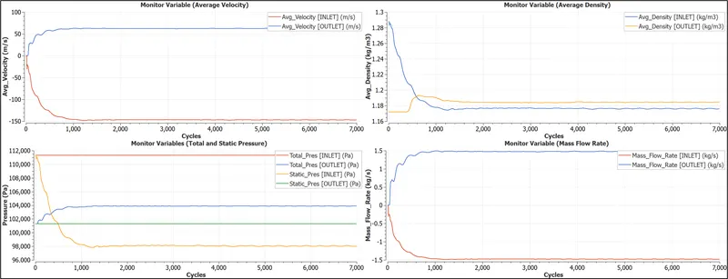
Fig. 5: Plots of monitor variables velocity, density, mass flow rate and pressure for steady-state simulation using RKE turbulence model for mesh 1

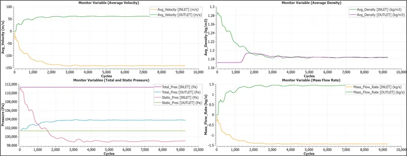
Fig. 6: Plots of monitor variables velocity, density, mass flow rate and pressure for steady-state simulation using RKE turbulence model for mesh 2

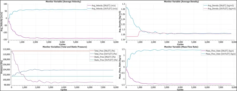
Fig. 7: Plots of monitor variables velocity, density, mass flow rate and pressure for steady-state simulation using RKE turbulence model for mesh 3

From Fig. 5, Fig. 6, and Fig. 7, we can notice that the monitor variables show a highly stable output with minimum variations well before they reach the end of total number of cycles specified in the 'End time' parameter under the 'General' tab of 'Simulation Parameters' settings under the 'Case Setup' tree as 15000 indicating that a steady-state solution has been obtained. Moreover, the converged state velocity at the outlet for all the different meshes was recorded, on average, to be around 60m/s to 63m/s which resembles quite closely with the velocity value estimated from initial assessments at 59.1898 m/s as mentioned in Section 2.3.3 Determination of flow velocity across the BFS domain, Reynolds number, Boundary layer thickness and First Cell Height.

3. Results

3.1 Velocity magnitude and pressure gradients values using field plots

Fig. 8 and Fig. 9 below shows the velocity magnitude and pressure gradients across the BFS model for different mesh sizes using field plots at the slice region created by orienting the plane normal to the flow direction as was specified in Section 2.4 Post-Processing. It can be observed that for the given scenario and with increase in the spatial resolution, the differences in both the velocity and pressure gradients with regards to the visualisation of viscous effects and pressure drop are almost similar and indifferentiable.

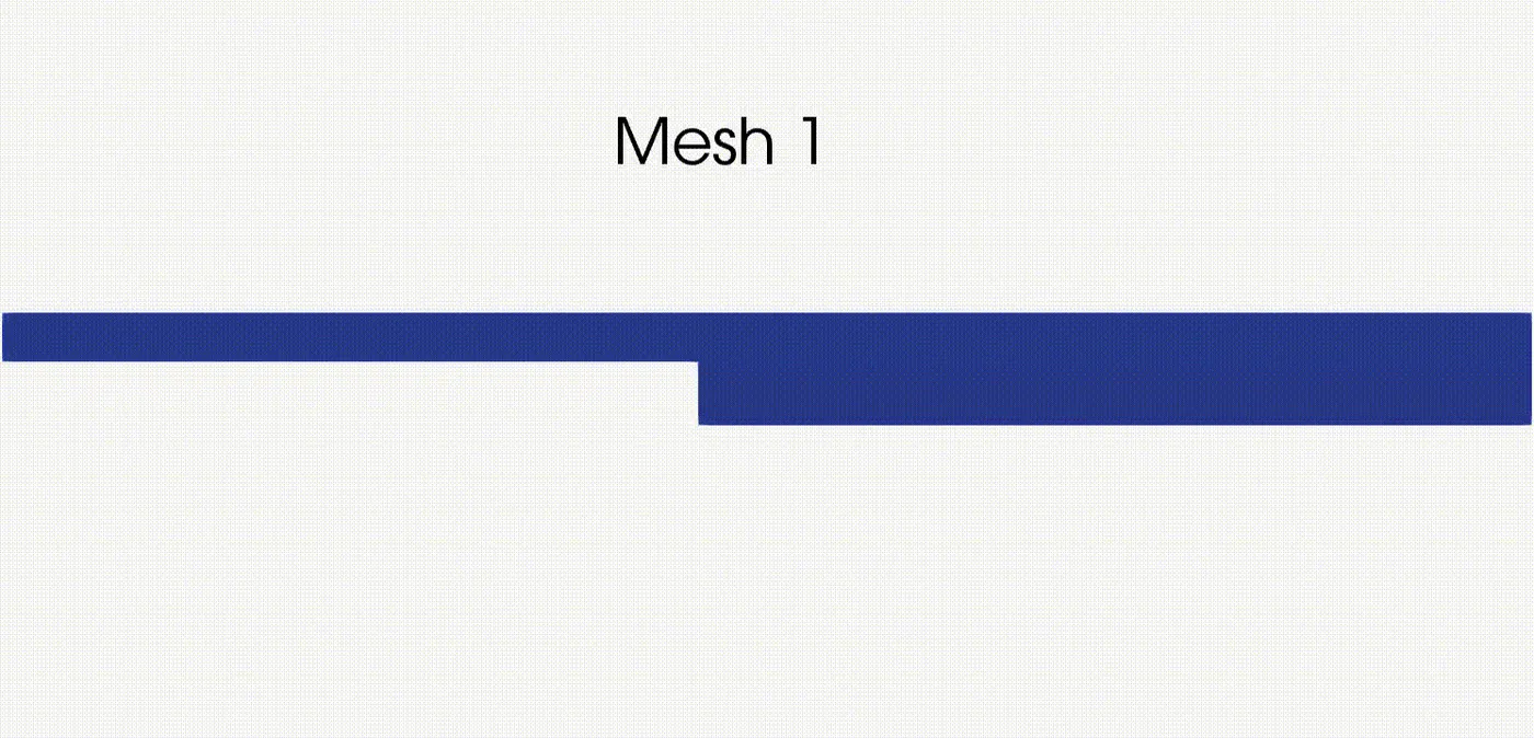
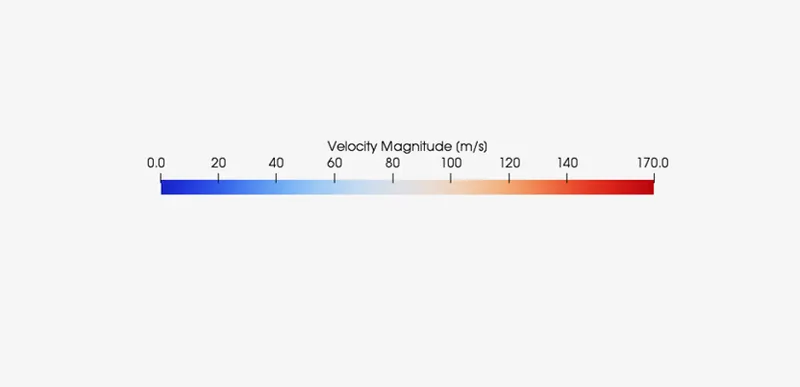Fig. 8: Velocity Magnitude field plots across the domain for different mesh sizes

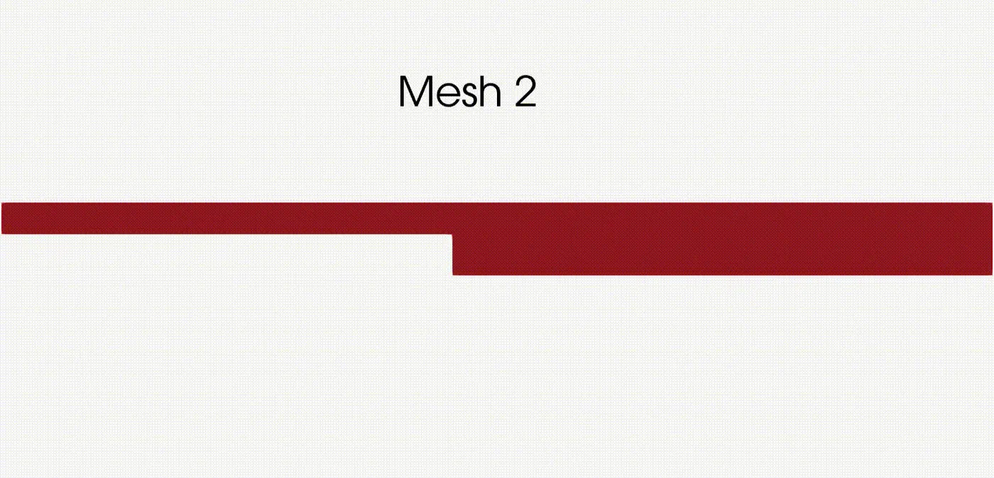
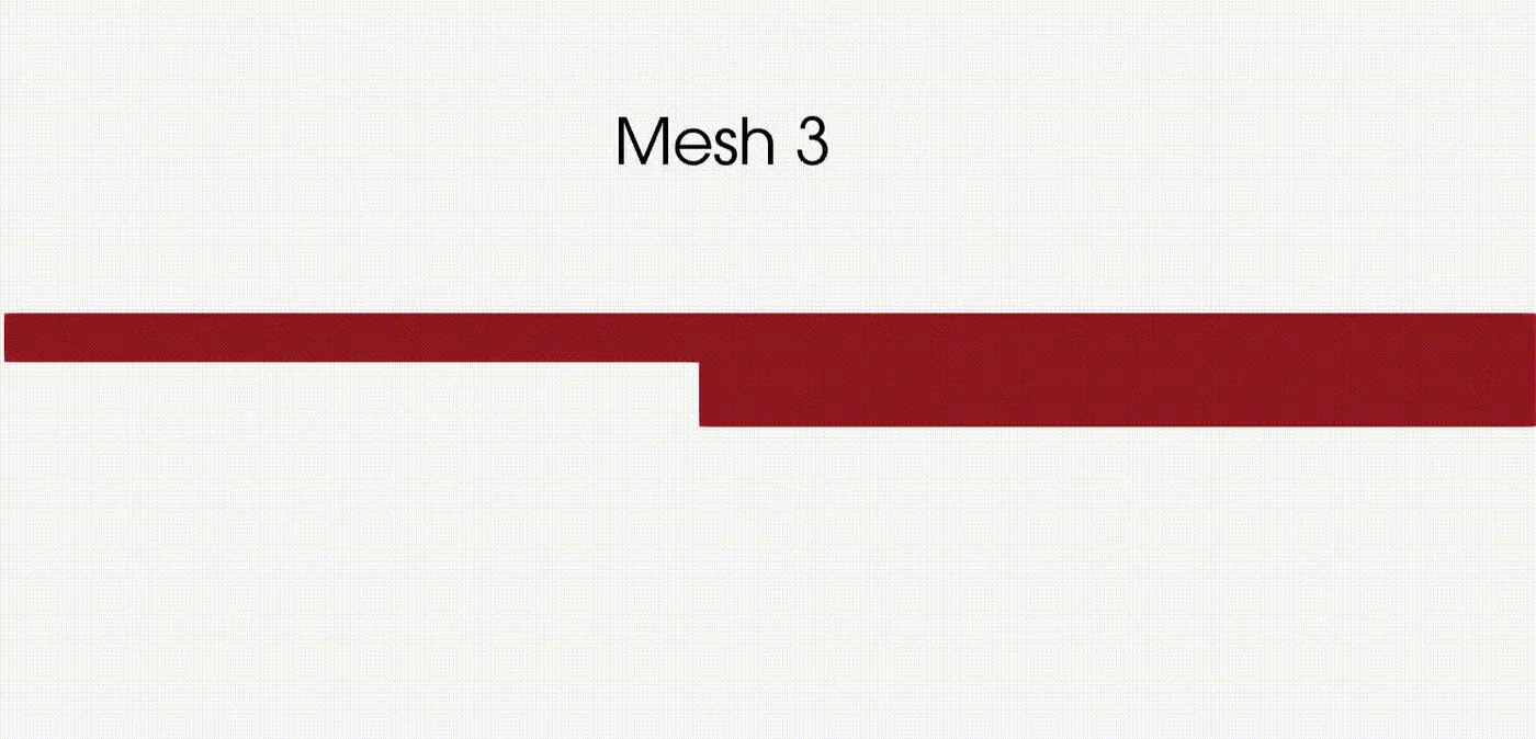
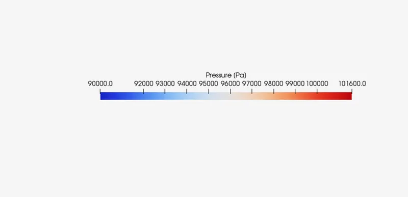
Fig. 9: Pressure field plots across the domain for different mesh sizes

3.2 Velocity magnitude and pressure drop values using line plots

The figures below i.e., Fig.10 and Fig. 11, shows the velocity magnitude and pressure drop profile plots at Line 1 and Line 2 respectively. It can be observed that for the velocity profiles, mesh 2 and mesh 3 have identical values as they approach towards the center of the inlet channel with almost similar peak magnitudes, as was also reported in Table 7, with the former also appearing to have reasonably good agreement with the analytical power-law velocity profile wherein the maximum velocity was calculated using the power-law velocity approach. Nevertheless, the numerical results and analytical solutions for the velocity magnitude profiles do not necessarily qualify for validation as the location at which the comparisons have been drawn does not represent the analytically determined fully-developed flow conditions as that position is located after the step wherein the velocity profiles, as a result of the sudden expansion, leads to rapidly decelerating flow and separation such that the velocity values close to the wall would no longer resemble the no-slip condition. The pressure drop plot showed similar behaviour as the velocity magnitude plot with mesh 2 and mesh 3 highlighting similar overall profiles.

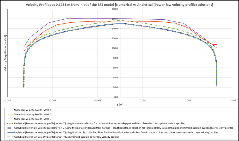
Fig. 10: Plot of comparison of velocity profiles between numerical and analytical (power-law) at 0.1231m from inlet of the BFS model at Line 1

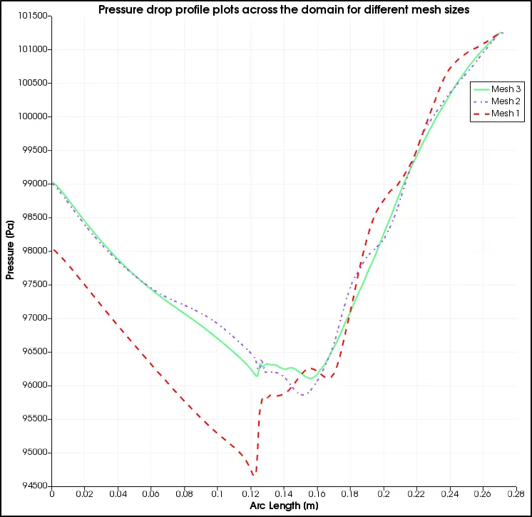
Fig. 11: Plot of Pressure drop profiles across the domain for different mesh sizes at Line 2

3.3 Comparison of law of the wall and logarithmic-law velocity profiles

Since, the gradients of the velocity field are varying by large magnitudes near the wall on account of the developing boundary layer, it was necessary to ensure that this region was properly resolved which in the given case was performed using the RKE turbulence model and a standard wall function approach such that the first grid cell was in the log-law layer or within the range of 30 < `y^+` < 300. Although, the location for the comparison of the law of the wall and logarithmic-law velocity profiles for mesh 2 (mesh independent result) does not lie at the empirically evaluated fully-developed flow condition for reasons indicated in Section 3.2 Velocity magnitude and pressure drop values using line plots i.e., the fully-developed flow condition is positioned after the step where the flow has separated, the position of the cell-centroid of the first grid cell in Fig. 12 clearly demonstrates that it lies in the log-law layer. Moreover, the layer closest to the wall (or the viscous sub-layer) was suggested by Prandtl [12] to be the zone wherein the velocity profile is linear such that the relation `u^+ = y^+` is obeyed, also confirmed by Nikuradse's experiments [13], usually upto `y^+ = 5` for smooth surfaces and similarly the logarithmic law-overlap layer, proposed by Von Karman [14], is the region wherein the velocity behaves as being directly proportional to the logarithm of the distance such that `u^+ = (1/kappa)ln y^+ + B`, typically in the range of 30 < `y^+` < 300, such that values of `kappa` and 'B' were experimentally evaluated as 0.42 [15] and 5.5 for smooth wall surfaces which in Converge are also known as 'Von Karman's constant' and 'Law of the wall parameter' respectively. A third layer exists as a region between the viscous sub-layer and the log-law layer, called as the Buffer layer, where both the viscous and turbulence effects occur but neither velocity profile from the other two regions are followed or are accurate to represent the ongoing physical effects with maximum deviation between the two velocity profiles occurring at the intercept position of around `y^+ = 11`, similar to the observation in Fig. 12 below. Investigations were carried out to describe a universal turbulent velocity behaviour in an attempt to fit Nikuradse's experimental data [13] near the wall such as the three-layer Karman model [16] represented by three separate algebraic equations for the three different layers in the inner region of the velocity profile, Reichardt's [17] and Spalding's [18] law of the wall models defined with single algebraic equations for `y^+>=0` with the latter showing comparable conformity with the given simulation results in the viscous sub-layer and log-law layer. It should be realised that the `u^+` vs `y^+` profiles as seen in Fig. 12 corresponding to the different layers in the inner region and the universal turbulent velocity behaviour were designed for incompressible fluid flow with values of its associated quantities belonging to the averaged and converged state conditions corresponding to last time-step size, however, in the given numerical simulation and based on Reynolds number of the hydraulic diameter of a non-circular cross-section, the flow is compressible and turbulent and therefore, they should be at best considered to be suggestive and not the real representation, including the value mentioned in the plot at the cell-centroid of the first grid cell as opposed to its actual value mentioned in Table 7, and while different formulations do exist for the compressible law of the wall, sufficient information about the wall temperatures, wall density and wall thermal conductivity among many others were not known at the time of performing the given numerical simulation.

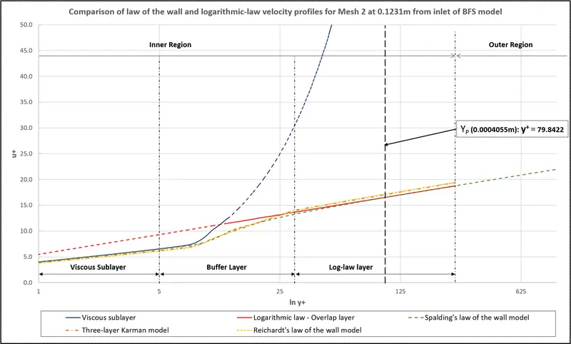
Fig. 12: Plot of comparison of law of the wall and logarithmic-law velocity profiles for Mesh 2 at 0.1231m from inlet of the BFS model and `y^+` value at distance from the cell-centroid 'P' to the wall (`y_P`)

3.4 Separation and Recirculation region

As mentioned previously in Section 3.2 Velocity magnitude and pressure drop values using line plots, the flow immediately after the step undergoes sharp deceleration due to the sudden expansion along with creation of an adverse pressure gradient such that the wall bounded flow gets separated beyond it leading to formation of a recirculation region and subsequent reattachment later downstream as seen in Fig. 13 below.

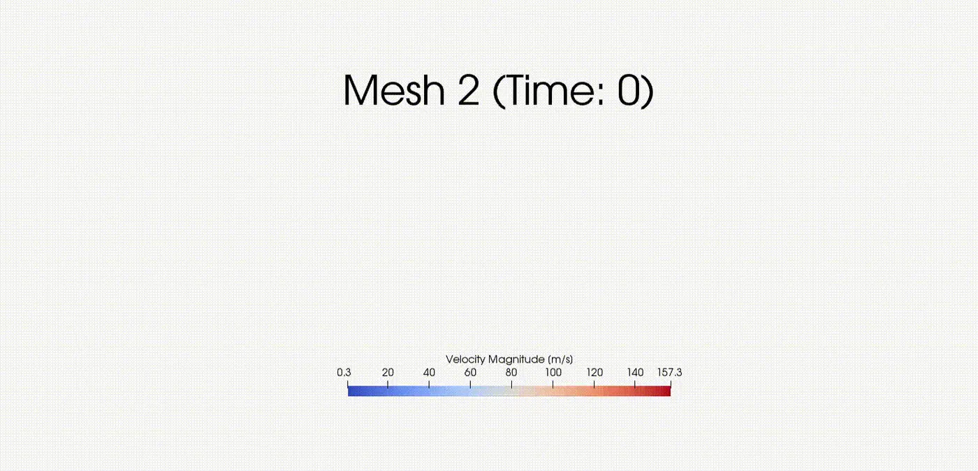
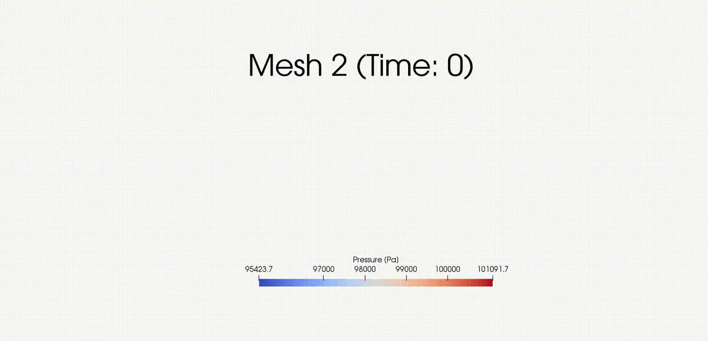
Fig. 13: Separation and recirculation regions near the step of BFS model for Mesh 2 with arrows oriented in a local velocity coloured (a) and pressure coloured (b) field plots

4. Discussion

Air enters at the inlet of the given cross-section of the BFS model, containing a mixture of two major contributing gas species `O_2` and `N_2` by mass fraction, as a turbulent flow resulting in the chaotic and unorganised mixing of fluid layers to form eddies that cause the transfer of mass and momentum to be enormously catalysed. The movement and intensity of eddies, however, decreases in intensity near the boundary walls as it travels downstream due to the "no slip" condition and effectively is confined away from it such that the turbulent boundary layer formed experiences a steep velocity gradient close to the wall but changes at a slower rate in its core region. This abrupt change in velocity values close to the wall tends to create wall shear stress of greater magnitudes than laminar flow through the same domain with a more fuller shape of the fully developed velocity profile appearing for the former as opposed to parabolic for the latter. As the wall-attached flow advances towards the step of the backward-facing step model, the sudden expansion in the domain cross-section causes the flow to decelerate such that pressure gradients increase creating a zone of unfavourable or adverse pressure gradient leading to flow separation. Consequently, a recirculation region is developed with reverse flow such that the developed boundary layer with an almost fuller turbulent profile is essentially disrupted and the boundary layer equations no longer remain valid. This zone of recirculation, also called as the separated region, is identified as a low-pressure region leading to the formation of a shear layer which eventually goes on to forming a reattachment point, depending on the length of the domain, where the flow gets reattached as a consequence of development of the unstable and large-scale turbulent structures beyond which a state of equilibrium for the turbulent boundary layer profile is achieved with no reverse flow.

5.Conclusion

The numerical analysis for flow within a BFS model under steady-state conditions using RKE turbulence model in Converge Studio v3.0 and executed using the Cygwin64 terminal was well understood. It was realised that based on the wall modelling approach of using a wall function and selecting appropriate `y^+` values, the turbulent or log-law region was well captured, albeit an approximation to the incompressible law of the wall model, along with visualisation of the flow separation and reattachment in the vicinity of the step. The determination of flow-field variables like velocity, density and pressure (total and/or static depending on the zone) from initial assessments also stressed the importance of assigning correct boundary and initial conditions as the final state or converged values especially at the outlet were remarkably close which greatly aided in selecting an appropriate solver and assessing the boundary layer profile growth. However, the CFD model would require further verification in terms of incorporating additional information about the compressibility effects and validation as part of an extended scope wherein the fully-developed flow conditions would preferably occur before the step of the backward-facing step model based on an appropriate Reynolds number.

References

[1] Driver, D. M. and Seegmiller, H. L., "Features of Reattaching Turbulent Shear Layer in Divergent Channel Flow," AIAA Journal, Vol. 23, No. 2, Feb 1985, pp. 163-171

[2] CONVERGE 3.0 Manual. © 2020 Convergent Science. All rights reserved. July 15, 2020.

[3] Shih, T.-H., Liou, W.W., Shabbir, A., Yang, Z., and Zhu, J., 1995, “A New - Eddy-Viscosity Model for High Reynolds Number Turbulent Flows - Model Development and Validation.”, Computers Fluids, 24(3):227-238

[4] The Engineering ToolBox, Speed of Sound in Air, www.engineeringtoolbox.com, viewed 10 June 2021, <https://www.engineeringtoolbox.com/air-speed-sound-d_603.html>

[5] Engineers Edge, LLC, Viscosity of air, Dynamic and Kinematic, www.engineersedge.com, viewed 10 June 2021, <https://www.engineersedge.com/physics/viscosity_of_air_dynamic_and_kinematic_14483.htm#:~:text=The%20viscosity%20of%20air%20depends,2%20%2Fs%20or%2014.8%20cSt.>

[6] The Engineering ToolBox, Ratio of Specific Heat of Gases, www.engineeringtoolbox.com, viewed 10 June 2021, <https://www.engineeringtoolbox.com/specific-heat-ratio-d_608.html>

[7] The Engineering ToolBox, Universal and Individual Gas Constants, www.engineeringtoolbox.com, viewed 10 June 2021, <https://www.engineeringtoolbox.com/individual-universal-gas-constant-d_588.html>

[8] BLASIUS, P. R. H. 1913. Das Aehnlichkeitsgesetz bei Reibungsvorgangen in Flüssigkeiten. Forschungsheft 131, 1-41

[9] Hinze, J. O., Turbulence, 2nd Ed., McGraw-Hill, New York, 1975

[10] Nikuradse, J. “Stroemungsgesetze in rauhen Rohren.” Ver. Dtsch. Ing. Forsch., 361, 1933

[11] D. Brkić and P. Praks, Unified friction formulation from laminar to fully rough turbulent flow, Applied Sciences (2018). 8 (11), article 2036 URL <https://www.scipedia.com/public/Brkic_2018a>

[12] L. Prandtl, "Uber die ausgebildete Turbulenz," Z. fur angew. Math. Mech., vol. 5,1925, p. 136

[13] J. Nikuradse, "Gesetzmiissigkeiten der turbulenten Stromung in glatten Rohren," Forschung a.d. Geb. Ing., No. 356, 1932.

[14] Von Karman, T. H. (1931). Mechanical similitude and turbulence. NACA Technical Memorandum 611.

[15] Kármán, Theodore von. 1930. “Mechanische Ähnlichkeit und Turbulenz.” Nachrichten von der Gesellschaft der Wissenschaften zu Göttingen, Mathematisch–Physikalische Klasse, 58–76.

[16] T. von Karman, "The Analogy Between Fluid Friction and Heat Transfer," Trans. ASME, vol. 61, 1939, pp. 705-710.

[17] H. Reichardt, "Vollstandige Darstellung der turbulenten Geschwindigkeitsverteilung in glatten Leitungen," Z. angew. Math. Mech., vol. 31, 1951, pp. 208-219

[18] Spalding, D.B. Heat Transfer to a Turbulent Stream from a Surface with a Step-wise Discontinuity in Wall Temperature. ASME Conference. Intern. Dev. in Heat Trans. Boulder, Colo. Part 11:439-466. 1961

[19] Moody, L.F. (1994). "Friction Factors for Pipe Flow". Transactions of the ASME. 66 (8): 671-684.