Week 7 - Simulation of a 1D Super-sonic nozzle flow simulation using Macormack Method
1. Introduction
Fluid flows and more specifically gas flowing through a conduit undergoes deflections against the walls of the conveying medium with velocity in the direction of flow typically increasing but density remaining the same as long as the local speed of flow is less than the local speed of sound within the same medium. This phenomena of the fluid is known as incompressibility, however, under conditions that the local speed of flow does approach the local speed of sound for the given medium, the gas begins to be affected by compressibility effects such that the density becomes a function of the position it is traversing. The same gas with the compressibility effects shows variations when travelling through different cross-sectional areas such that for a converging section i.e., decrease in area, the gas gets compressed while in a diverging section or increase in area, the same gas expands, and this can be controlled for the flow to restore to its original conditions or essentially return to its initial conditions. Since this process indicates its reversibility and if the flow were to be also adiabatic, then according to the second law of thermodynamics, a constant entropy value is maintained and this type of flow is distinguished as an isentropic flow. Applications of a steady, uniform and isentropic flow are commonly dealt with in flow though jet engine and nozzle of a rocket, flow past turbine blades, and these have great engineering significance as such devices are complex to build and present tremendous challenges requiring careful attention towards calculating the many variables that would define its success in difficult environmental situations. One such type of flow that has been discussed in the given numerical problem refers to the steady, isentropic flow through a convergent-divergent nozzle in which the flow to the nozzle inlet is delivered from a reservoir. The flow variables within the reservoir viz., pressure and temperature, are defined at certain values, however, due to the rather large cross-sectional area of the reservoir, the velocity of the flow tends to 0, and the same variables of pressure and temperature can also be referred to as stagnation values or total pressure and total temperature respectively. The flow undergoes isentropic expansion to supersonic speeds as it travels through the nozzle medium to the exit such that the flow is locally subsonic in its convergent section, sonic at its throat area, and supersonic in its divergent section with sonic indicating that local flow velocity is equivalent to the local speed of sound. For simplicity in defining an engineering model of the given flow, it was assumed that the flow properties along a cross-sectional area are constant and its variations are considered only along the linear distance in x-direction. This type of assumption wherein the flow problem is reduced from a two or three dimensional problem, for a simplified analysis, to a one-dimensional analysis can be referred to as a quasi-one-dimensional flow problem.
The aim of this programming exercise was to simulate the quasi 1D isentropic flow through a subsonic-supersonic nozzle wherein both the conservation and non-conservation forms of the governing equations were solved using the MacCormack's technique. Additionally, the objectives also included evaluation of the time-wise variations and steady-state distributions for the non-dimensional representation of flow-field variables, Mach number and mass flow, and comparison between the same based on the two forms of governing equations also subjected to a grid independence test.
2. Method
2.1 Modelling
The problem was solved by building a mathematical model in Matlab (code snippet for which is attached with this report). Since, the domain was assumed to represent a quasi-one-dimensional flow problem, the number of grid points were defined along the x-axis direction only using the 'linspace' function which were linearly and equidistantly spaced by passing the domain length value of 3m representing the distance between the nozzle end points. The number of grid points were selected as 31 and 61, as was demonstrated in John D. Anderson, Jr., (1995), with regards to performing the grid independence test. The values for time-step size were calculated based on the stability analysis for an explicit numerical scheme represented by a linear hyperbolic equation such that the Courant number resulted in a value of less than 1, in this case as 0.5, with total number of time-steps assigned as 1400. Additionally, the ratio of specific heats i.e., `gamma = C_p/C_v` was set at the value of '1.4', assuming for air at standard conditions, determination of exact analytical solutions for non-dimensional primitive variables of pressure, density and temperature were based on the Area-Mach number relation and initial and boundary conditions as provided in John D. Anderson, Jr., (1995) with formulations and descriptions of the governing equations and MacCormack's technique explained in detail in Section 2.2 Mathematical Model Setup, of this report.
2.2 Mathematical Model Setup
2.2.1 Derivation of conservation and non-conservation form of governing equations using non-dimensional primitive variables (John D. Anderson, Jr., 1995)
In accordance with observing the overall physical principles of mass conservation, Newton's second law and conservation of energy, such that they are satisfied in the case of the given numerical problem, integral form of governing equations were applied to the control volume compatible with the assumptions for the same.
Integral form of continuity equation can be represented as:
`del/(del t)int int int_vartheta rho*dvartheta + int int_S rho*V*dS = 0` ;where (Eq. 1)
`rho`, `vartheta`, and 'S' represents density, volume, and surface area with the latter two also rewritten to indicate their integrals
The above (Eq. 1) is applied to the shaded control volume region represented in Fig. 1, which is of infinitesimal thickness 'dx'. The variables, pressure (p), velocity (V), density (`rho`) and energy (e), as part of the governing equations for the given flow problem on the left hand side of the control volume are uniform over the area (A) while the same terms i.e., pressure, velocity, density and energy designated by (p+dp), (V+dV), (`rho`+d`rho`) and (e+de) are uniform over the area (A+dA) on the right hand side of the control volume. As the limit 'dx' becomes increasingly small, the time derivative of the volume integral i.e., the first term in (Eq. 1) can be further simplified as:
`del/(del t)int int int_vartheta rho*dvartheta = del/(del t)(rho*A*dx)` ;where (Eq. 2)
'A*dx' is the volume of the control volume as 'dx' becomes infinitesimally smaller
Similarly, the surface integral term i.e., the second term in (Eq. 1), can also be further simplified as follows:
`int int_S rho*V*dS = -rho*V*A + (rho+drho)(V+dV)(A+dA)` (Eq. 3)
The mass flow term i.e., first term on the right hand side of (Eq. 3) is represented by a negative sign owing to vectors V and dS oriented in opposite directions to each other over the left face of the control volume leading to a negative dot product. The terms on the right hand side in (Eq. 3) can be expanded for further simplification as shown below:
`int int_S rho*V*dS = -rho*V*A + rho*V*A + rho*V*dA + rho*A*dV + rho*dV*dA + A*V*drho + V*dA*drho + A*dV*drho + drho*dV*dA`(Eq. 4)
As the limit 'dx' becomes infinitesimally smaller, the terms involving products of differentials approach 0 a lot quicker as opposed to terms containing only a single differential. Therefore, terms with products of differentials can be ignored from (Eq. 4) such that the resulting equation formed can be rewritten as follows:
`int int_S rho*V*dS = rho*V*dA + rho*A*dV + A*V*drho = d(rho*A*V)` (Eq. 5)
Substituting the simplified equations obtained for the volume and surface integrals from (Eq. 2) and (Eq. 5) respectively into (Eq. 1), we get
`del/(del t)(rho*A*dx) + d(rho*A*V) = 0` (Eq. 6)
Dividing (Eq. 6) by 'dx' throughout such that `(d(rho*A*V))/dx` represents the partial derivative with respect to x as 'dx' becomes infinitesimally smaller, we get
`del/(del t)(rho*A) + del/(del x)(rho*A*V) = 0` (Eq. 7)
The above (Eq. 7) represents the conservation form of the continuity equation that is acceptable for the given numerical problem as mass is conserved for the same. An equivalent non-conservative form of the continuity equation exists can be expressed by expanding (Eq. 7) to be mathematically written as:
`del/(del t)(rho*A) + rho*A*(del V)/(del x) + rho*V*(del A)/(del x) + V*A*(del rho)/(del x) = 0` (Eq. 8)

Fig. 1: Control Volume region for derivation of partial differential equations for the unsteady, quasi one-dimensional flow (Image recreated for this study as illustrated in John D. Anderson, Jr., (1995) with no intention to infringe on the copyrights of the original author and/or his publication)
Similarly, the integral form of the x-component of the momentum equation for an inviscid flow i.e., neglecting the viscous stress terms, with no body forces can be expressed as shown below:
`del/(del t)int int int_vartheta (rho*u)*dvartheta + int int_S (rho*u*V)*dS = -int int_S (p*dS)_x` ;where (Eq. 9)
`(p*dS)_x` signifies the x component of the vector `(p*dS)`
Implementing the above (Eq. 9), similar to the continuity equation in (Eq. 1), to the shaded control volume in Fig. 1, we obtain the volume and surface integrals as shown below:
`del/(del t)int int int_vartheta (rho*u)*dvartheta = del/(del t)(rho*V*A*dx)` , and (Eq. 10)
`int int_S (rho*u*V)*dS = -rho*V^2*A + (rho+drho)(V+dV)^2(A+dA)` (Eq. 11)
In order to evaluate the pressure force term on the right hand side of (Eq. 9) can be better understood with Fig. 2 wherein the x components of the vector `(p*dS)` has been illustrated on all four sides of the control volume with the fact that the surface derivative `(dS)` always directs away from the control volume and therefore any x component i.e., `(p*dS)_x` that is aligned in the left or negative x direction is a negative quantity whereas the same term along the same component aligned in the right or positive x direction is a positive quantity. It should also be noted that the x component of the vector `(p*dS)` i.e., `(p*dS)_x` directed on the top and bottom inclined faces of the control volume are represented as pressure term acting on the component of the inclined area extended perpendicular to the x direction or `(dA)/2` and subsequently the addition of each inclined face to the pressure integral term is `-p*(dA)/2`. In other words, the right hand side of (Eq. 9) can now be expressed as:
`-int int_S (p*dS)_x = -p*A + (p+dp)(A+dA)-2*p*((dA)/2)` (Eq. 12)
Substituting (Eq. 10), (Eq. 11) and (Eq. 12) into (Eq. 9), we get
`del/(del t)(rho*V*A*dx) + -rho*V^2*A + (rho+drho)(V+dV)^2(A+dA) = p*A - (p+dp)(A+dA) + p*dA` (Eq. 13)
Removing like terms and ignoring products of differentials as done in (Eq. 5) since limit 'dx' becomes infinitesimally smaller, we get
`del/(del t)(rho*V*A*dx) + d(rho*V^2*A) = -A*dp` (Eq. 14)
Dividing (Eq. 14) by 'dx' throughout such that `(d(rho*V^2*A))/dx` represents the partial derivative with respect to x as 'dx' becomes infinitesimally smaller, similar to (Eq. 7), we get
`del/(del t)(rho*V*A) + del/(del x)(rho*V^2*A) = -A*(del p)/(del x)` (Eq. 15)
The above (Eq. 15) represents the x component of momentum equation in the conservative form. An equivalent non-conservation form of the x component of momentum equation is also obtainable by multiplying the continuity equation represented in (Eq. 7) by `V` such that the same equation can be expressed as shown below:
`V*del/(del t)(rho*A) + V*del/(del x)(rho*A*V) = 0` (Eq. 16)
(Eq. 16) is then subtracted from (Eq. 15) such that the equations now appears as:
`del/(del t)(rho*V*A) - V*del/(del t)(rho*A) + del/(del x)(rho*V^2*A) - V*del/(del x)(rho*A*V) = -A*(del p)/(del x)` (Eq. 17)
Simplifying (Eq. 17) by expanding derivatives on its left hand side, cancelling the like terms and dividing by 'A' throughout, we get
`rho*(del V)/(del t) + rho*V*(del V)/(del x) = -(del p)/(del x)` (Eq. 18)
(Eq. 18) represents the x component of momentum equation in the non-conservative form.
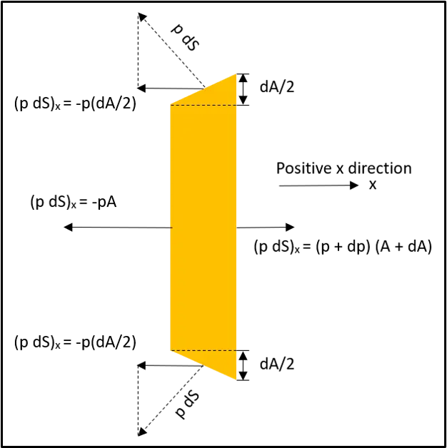
Fig. 2: Forces acting along either direction of the x-axis subjected on the control volume (Image recreated for this study as illustrated in John D. Anderson, Jr., (1995) with no intention to infringe on the copyrights of the original author and/or his publication)
Lastly, we derive the conservative and non-conservative forms of the energy equation from its integral form developed for an adiabatic flow (or `dot q = 0`) having no body forces and no viscous effects which is expressed as shown below:
`del/(del t)int int int_vartheta rho*(e+V^2/2)*dvartheta + int int_S rho*(e+V^2/2)*V*dS = -int int_S (p*V)*dS` ;where (Eq. 19)
Applying the above (Eq. 19), similar to the x-component of the momentum equation in (Eq. 9), to the shaded control volume in Fig. 1 while being aware of the pressure forces as highlighted in Fig. 2, we obtain:
`del/(del t)[ rho*(e+V^2/2)*A*dx] - rho*(e+V^2/2)*V*A + (rho + drho)*[e + de + (V+dV)^2/2]*(V+dV)*(A+dA) = -[-p*V*A + (p+dp)*(V+dV)*(A+dA) - 2*(p*V*(dA)/2)]` (Eq. 20)
Cancelling like terms and ignoring products of differentials as done in (Eq. 14) since limit 'dx' becomes infinitesimally smaller, we get
`del/(del t)[ rho*(e+V^2/2)*A*dx] + d(rho*e*V*A) + (d(rho*V^3*A))/2 = -d(p*A*V)` ;where (Eq. 21)
OR
`del/(del t)[ rho*(e+V^2/2)*A*dx] + d(rho*(e+V^2/2)*V*A) = -d(p*A*V)` ;where (Eq. 22)
Dividing (Eq. 22) by 'dx' throughout such that `(d(rho*(e+V^2/2)*V*A))/dx` represents the partial derivative with respect to x as 'dx' becomes infinitesimally smaller, similar to (Eq. 15), we get
`del/(del t)[ rho*(e+V^2/2)*A*dx] + del/(del x)(rho*(e+V^2/2)*V*A) = -del/(del x)(p*A*V)` ;where (Eq. 23)
The above (Eq. 23) represents the conservation form of energy expressed in total energy terms `(e+V^2/2)`. The same energy equation can be expressed in terms of internal energy by multiplying the x component of momentum equation represented in (Eq. 15) by `V` as shown below:
`del/(del t)(rho*(V^2/2)*A) + del/(del x)(rho*(V^3/2)*A) = -A*V*(del p)/(del x)` (Eq. 24)
(Eq. 24) is then subtracted from (Eq. 23) such that the equations now appears as:
`del/(del t)(rho*e*A) + del/(del x)(rho*e*V*A) = -p*(del (A*V))/(del x)` (Eq. 25)
The above (Eq. 25) represents the conservation form of energy expressed in internal energy terms `e`. An equivalent non-conservation form of the energy equation expressed in internal energy terms is also obtainable by multiplying the continuity equation represented in (Eq. 7) by `e` such that the same equation can be expressed as shown below:
`e*del/(del t)(rho*A) + e*del/(del x)(rho*A*V) = 0` (Eq. 26)
Subtracting (Eq. 26) from (Eq. 25) such that the equations now appears as:
`rho*A*(del e)/(del t) + rho*A*V*(del e)/(del x) = -p*del/(del x)(A*V)` (Eq. 27)
Expanding the terms on the right hand side of (Eq. 27) and dividing by 'A' throughout, we get
`rho*(del e)/(del t) + rho*V*(del e)/(del x) = -p*(del V)/(del x) -p*(V/A)(del A)/(del x)` (Eq. 28)
OR
`rho*(del e)/(del t) + rho*V*(del e)/(del x) = -p*(del V)/(del x) -p*V*(del (ln A))/(del x)` (Eq. 29)
(Eq. 29) represents the non-conservative form of energy equation expressed in terms of internal energy.
The requirement of establishing the energy equation in terms of internal energy arises from the fact that for a calorically perfect gas, both conservative and non-conservative forms of energy equation expressed in (Eq. 25) and (Eq. 29) respectively, can also be rewritten in terms of temperature 'T'. Since, in the case of the given numerical problem, the assumption of a calorically perfect gas was to be investigated, the relation between the dependent variable 'e' and fundamental or independent variable 'T' can be expressed as shown below:
`e = C_v*T` (Eq. 30)
Substituting (Eq. 30) into (Eq. 29) and rewriting the same, we get
`rho*C_V(del T)/(del t) + rho*V*C_V*(del T)/(del x) = -p*(del V)/(del x) -p*V*(del (ln A))/(del x)` (Eq. 31)
To summarise, (Eq. 8), (Eq. 18) and (Eq. 31) represent the continuity, x component of momentum and energy equations in non-conservative form indicating that the resulting number of equations are three, however, the number of unknown variables are four i.e., `rho`, 'V', 'p' and 'T'. Therefore, we need to resolve the mismatch or imbalance in order to obtain a unique solution which in this case is achieved by revisiting the equation of state as shown below:
`p = rho*R*T` (Eq. 32)
Also, the spatial derivative of the same equation of state along x direction as shown in (Eq. 32) can be attained as follows:
`(del p)/(del x) = R*(rho*(del T)/(del x) + T*(del rho)/(del x))` (Eq. 33)
This implies from (Eq. 32) and (Eq. 33) that the pressure term can be eliminated from (Eq. 18) and (Eq. 31) such that they can be rewritten as shown below:
Momentum (x component): `rho*(del V)/(del t) + rho*V*(del V)/(del x) = -R*(rho*(del T)/(del x) + T*(del rho)/(del x))` (Eq. 34)
Energy: `rho*C_V(del T)/(del t) + rho*V*C_V*(del T)/(del x) = -rho*R*T*[(del V)/(del x) +V*(del (ln A))/(del x)]` (Eq. 35)
(Eq. 34) and (Eq. 35) represent the x component of momentum, and energy equations respectively in the non-conservative form expressed using the fundamental variables. However, quite often and especially with nozzle based flows, the aforementioned equations of continuity, x component of momentum and energy expressed for the non-conservative form using the fundamental variables are also represented in their non-dimensional aspects wherein the flow variables are referenced with respect to the reservoir values from where they originate i.e., of the format `p/p_0`, `rho/rho_0`, and `T/T_0` such that their values vary between 0 and 1, in other words the quantities are normalised to enable better visualisation of the concerned profiles. Therefore, in order to rewrite the non-conservative form of the governing equations using the non-dimensional approach, the normalised variables have been defined as follows:
Dimensionless Temperature: `T' = T/T_0` (Eq. 36)
Dimensionless Density: `rho' = rho/rho_0` (Eq. 37)
Dimensionless Length: `x' = x/L` (Eq. 38)
Dimensionless Velocity: `V' = V/a_0` (Eq. 39)
Dimensionless Time: `t' = t/(L/a_0)` (Eq. 40)
Dimensionless Area: `A' = A/A^(star)` (Eq. 41)
(Eq. 36) to (Eq. 41) represent the non-dimensional terms of the various quantities that would be used to represent the non-dimensional form of the governing equations beginning with the non-conservative form of the same wherein `a_0` indicates the speed of sound in reservoir which is equivalent to the square root of the product of ratio of specific heats, gas constant and temperature in the reservoir i.e., `sqrt(gamma*R*T_0)` and `A^(star)` represents the sonic throat area. Rewriting the non-conservative form of continuity equation expressed in (Eq. 8) using the non-dimensional terms from (Eq. 36) to (Eq. 41), we get
`(del rho'*A')/(del t')*((rho_0*A^(star))/(L/a_0)) + rho'*A'*(del V')/(del x')*((rho_0*A^(star)*a_0)/L) + rho'*V'*(del A')/(del x')*((rho_0*A^(star)*a_0)/L) + V'*A'*(del rho')/(del x')*((a_0*A^(star)*rho_0)/L) = 0`(Eq. 42)
Since, nozzle geometry is a function of x and not time or in other words is independent of the latter, therefore the time derivative seen as the first time on the left hand side of (Eq. 42) can be simplified as seen below:
`(del (rho'*A'))/(del t) = A'*(del rho')/(del t)` (Eq. 43)
Substituting the simplification as seen in (Eq. 43) into (Eq. 42), we get the continuity equation in non-dimensional form as shown below:
`(del rho')/(del t) = - rho'*(del V')/(del x') - rho'*V'*(del (ln A'))/(del x') - V'*(del rho')/(del x')` (Eq. 44)
Similarly, rewriting the non-conservative form of the x component of momentum equation expressed in (Eq. 34) using the non-dimensional terms from (Eq. 36) to (Eq. 41), we get
`rho'*(del V')/(del t')*((rho_0*a_0)/(L/a_0)) + rho'*V'*(del V')/(del x')*((rho_0*a_0^2)/L) = -R*(rho'*(del T')/(del x') + T'*(del rho')/(del x'))*((rho_0*T_0)/L)` (Eq. 45)
OR
`rho'*(del V')/(del t') = -rho'*V'*(del V')/(del x') -(rho'*(del T')/(del x') + T'*(del rho')/(del x'))*((R*T_0)/a_0^2)` (Eq. 46)
The term `((R*T_0)/a_0^2)` can be simplified such that it can be expressed in terms of ratio of specific heats as shown below:
`(R*T_0)/(a_0^2) = (gamma*(R*T_0))/(gamma*a_0^2) = (a_0^2)/(gamma*a_0^2) = 1/gamma` (Eq. 47)
Substituting the simplified version of the term `((R*T_0)/a_0^2)` as shown in (Eq. 47) into (Eq. 46), we get the x component of momentum equation in non-dimensional form as shown below:
`(del V')/(del t') = -V'*(del V')/(del x') -(1/gamma)*((del T')/(del x') + (T')/(rho')*(del rho')/(del x'))` (Eq. 48)
Finally, rewriting the non-conservative form of the energy equation expressed in (Eq. 35) using the non-dimensional terms from (Eq. 36) to (Eq. 41), we get
`rho'*C_V(del T')/(del t')*((rho_0*T_0)/(L/a_0)) + rho'*V'*C_V*(del T')/(del x')*((rho_0*a_0*T_0)/L) = -rho'*R*T'*[(del V')/(del x') +V'*(del (ln A'))/(del x')]*((rho_0*T_0*a_0)/L)` (Eq. 49)
In the above (Eq. 49), the factor `R/C_v` can also be given as:
`R/C_V = R/(R/(gamma-1)) = gamma-1` (Eq. 50)
Substituting the above relation of `R/C_v` from (Eq. 50) into (Eq. 49), we get the energy equation in non-dimensional form as shown below:
`(del T')/(del t') = - V'*(del T')/(del x') - (gamma-1)*T'*[(del V')/(del x') +V'*(del (ln A'))/(del x')]` (Eq. 51)
The above steps performed with regards to obtaining the non-conservative form of governing equations by normalising it using (Eq. 36) to (Eq. 41) have been repeated to obtain the conservative form of governing equations starting with the continuity equation, as seen in (Eq. 7), shown below:
`del ((rho/rho_0*A/A^(star)))/(del (t/(L/a_0)))((rho_0*A^(star)*a_0)/L) + del ((rho/rho_0*A/A^(star)*V/a_0))/(del (x/L))((rho_0*A^(star)*a_0)/L) = 0` (Eq. 52)
OR
`(del (rho'*A'))/(del t') + (del (rho'*A'*V'))/(del x') = 0` (Eq. 53)
Similarly, the conservative form of x component of momentum equation, as seen in (Eq. 15), can be arrived at in its non-dimensional form by first implementing the chain rule to the term on the right hand side of the same equation i.e., (Eq. 15), followed by using (Eq. 36) to (Eq. 41), both of which have been shown below:
`(del (p*A))/(del x) = p (del A)/(del x) + A (del p)/(del x)` (Eq. 54)
Substituting the terms in (Eq. 53) such that the term `A (del p)/(del x)` is moved to its left hand side, into (Eq. 15), we obtain
`del/(del t)(rho*V*A) + del/(del x)(rho*V^2*A + p*A) = p*(del A)/(del x)` (Eq. 55)
Creating the non-dimensional form of the above (Eq. 55), we get
`(del (rho/rho_0*A/A^(star)*V/a_0))/(del (t/(L/a_0)))((rho_0*A^(star)*a_0^2)/L) + (del [rho/rho_0*A/A^(star)*V^2/a_0^2*rho_0*A^(star)*a_0^2 + p/p_0*A/A^(star)*(p_0*A^(star))])/(del (x/L)*L) = p/p_0*(del (A/A^(star)))/(del(x/L))*((p_0*A^(star))/L)` (Eq. 56)
OR
`(del (rho'*A'*V'))/(del t') + (del [rho'*A'*V'^2 + p'*A'*(p_0/(rho_0*a_0^2))])/(del x') = p'*(del A')/(del x')*(p_0/(rho_0*a_0^2))` (Eq. 57)
The term `(p_0/(rho_0*a_0^2))` in (Eq. 57) can be further simplified in terms of gamma as shown below:
`p_0/(rho_0*a_0^2) = (rho_0*R*T_0)/(rho_0*a_0^2) = (rho_0*R*T_0)/(rho_0*gamma*R*T_0) = 1/gamma` (Eq. 58)
Substituting the above transformation of the term `(p_0/(rho_0*a_0^2))` in (Eq. 58) into (Eq. 57), we obtain the conservative form of x component of momentum equation in non-dimensional terms:
`(del (rho'*A'*V'))/(del t') + (del [rho'*A'*V'^2 + (1/gamma)*p'*A'])/(del x') = (1/gamma)*p'*(del A')/(del x')` (Eq. 59)
Lastly, the conservative form of energy equation in terms of total energy, as seen in (Eq. 23), can be arrived at in its non-dimensional form by first combining the spatial derivatives in the x direction of the same equation i.e., (Eq. 23), followed by defining the non-dimensional energy term and then using (Eq. 36) to (Eq. 41) to obtain the concerned equation using non-dimensional primitive variables, all of which has been shown below:
`del/(del t)[ rho*(e+V^2/2)*A*dx] + del/(del x)(rho*(e+V^2/2)*V*A + p*A*V) = 0` (Eq. 60)
A non-dimensional form of internal energy term, `e`, can be defined as follows:
`e' = e/e_0; e_0 = C_V*T_0 = (R*T_0)/(gamma - 1)` (Eq. 61)
Substituting the above relation of non-dimensional form of internal energy in (Eq. 61) into (Eq. 60), we get
`(del {rho/rho_0*[e/e_0*(e_0)+V^2/(2*a_0^2)*(a_0^2)]*A/A^(star)})/(del (t/(L/a_0)))*((rho_0*A^(star)*a_0)/L) + (del {rho/rho_0*[e/e_0*(e_0)+V^2/(2*a_0^2)*(a_0^2)]*V/a_0*A/A^(star)*(rho_0*a_0*A^(star))+(p/p_0*A/A^(star)*V/a_0)*p_0*A^(star)*a_0})/(del (x/L)*L) = 0` (Eq. 62)
As `e_0 = (R*T_0)/(gamma - 1)`, (Eq.62) can be transformed in terms of non-dimensional primitive variables as shown below:
`(del [rho'*((e')/(gamma-1)+gamma/2*V'^2)*A'])/(del t')*((rho_0*A^(star)*a_0*R*T_0)/L) + (del [rho'*((e')/(gamma - 1)+gamma/2*V'^2)*V'*A'*((rho_0*a_0*A^(star)*R*T_0)/L)+(p'*A'*V')*((p_0*A^(star)*a_0)/L)]]/(del x') = 0` (Eq. 63)
Dividing (Eq. 63) by `((rho_0*A^(star)*a_0*R*T_0)/L)` throughout, we get
`(del [rho'*((e')/(gamma-1)+gamma/2*V'^2)*A'])/(del t') + (del [rho'*((e')/(gamma - 1)+gamma/2*V'^2)*V'*A'+(p'*A'*V')*(p_0/(rho_0*R*T_0))]]/(del x') = 0` (Eq. 64)
However, from equation of state expressed in (Eq. 32), we get
`p_0/(rho_0*R*T_0) = (rho_0*R*T_0)/(rho_0*R*T_0) = 1` (Eq. 65)
Substituting the above relation obtained in (Eq. 65) back into (Eq. 64), we get the non-dimensional conservative form of the energy equation:
`(del [rho'*((e')/(gamma-1)+gamma/2*V'^2)*A'])/(del t') + (del [rho'*((e')/(gamma - 1)+gamma/2*V'^2)*V'*A' + p'*A'*V']]/(del x') = 0` (Eq. 66)
(Eq. 53), (Eq. 59) and (Eq. 66) represent the non-dimensional conservative forms of continuity, x component of momentum and energy equations, however, they can be made generic similar to the governing equations for unsteady, three-dimensional flow by forming solutions vectors 'U', flux vectors 'F' and source term vector 'J' as shown below:
`U1 = rho'*A'` (Eq. 67)
`U2 = rho'*A'*V'` (Eq. 68)
`U3 = rho'*((e')/(gamma - 1)+gamma/2*V'2)A'` (Eq. 69)
`F1 = rho'*A'*V'` (Eq. 70)
`F2 = rho'*A'*V'^2+1/gamma*p'*A'` (Eq. 71)
`F3 = rho'*((e')/(gamma - 1)+gamma/2*V'^2)A' + p'*A'*V'` (Eq. 72)
`J2 = 1/gamma*p'*(del A')/(del x')` (Eq. 73)
Based on the elements used above from (Eq. 67) to (Eq. 72), the non-dimensional conservative forms of continuity, x component of momentum and energy equations can be rewritten as:
Continuity: `(del U1)/(del t') = -(del F1)/(del x')` (Eq. 74)
Momentum (x component): `(del U2)/(del t') = -(del F2)/(del x') + J2` (Eq. 75)
Energy: `(del U3)/(del t') = -(del F3)/(del x')` (Eq. 76)
(Eq. 74) to (Eq. 76) above represent the continuity, x component of momentum and energy equations that would be used to obtain numerical solution based on the MacCormack's technique, however, these equations are expressed in terms of solution vectors and not the primitive variables which would give a better understanding of the physical problem in context. Therefore, to obtain the non-dimensional solutions in terms of the fundamental variables, the elements representing the solutions vectors viz., U1, U2 and U3 need to decoded as shown below:
`rho' = (U1)/(A')` (Eq. 77)
`V' = (U2)/(U1)` (Eq. 78)
`T' = e' = (gamma - 1)*((U3)/(U1)-gamma/2*V'^2)` (Eq. 79)
`p' = rho'*T'` (Eq. 80)
It was observed by John D. Anderson, Jr., (1995), that whenever the flux vectors were expressed in terms of the non-dimensional primitive variables, as seen from (Eq. 70) to (Eq. 72), it was recorded by John D. Anderson, Jr., (1995) and in the light of the given numerical problem that instabilities tend to arise in the subsonic section of the nozzle and beyond the 300 time steps mark, the solution blows up or in other words erratic divergence takes place and it was ascertained that this behaviour was predominantly based on the lack of "purity" with which the conservative form of governing equations were being formulated as seen in (Eq. 74) to (Eq. 76) that the dependent variables are the solutions vectors and not the primitive variables. Therefore, based on John D. Anderson, Jr., (1995) suggestion, (Eq. 74) to (Eq. 76) was expressed with regards to the dependent variables i.e., the solutions vectors, and not the primitive variables as shown below:
`F1 = F1(U1,U2,U3)` (Eq. 81)
`F2 = F2(U1,U2,U3)` (Eq. 82)
`F3 = F3(U1,U2,U3)` (Eq. 83)
`J2 = J2(U1,U2,U3)` (Eq. 84)
On a close comparison between (Eq. 70) and (Eq. 68), it can be deduced that
`F1 = U2` (Eq. 85)
Similarly, comparing (Eq. 71), and (Eq. 67) to (Eq. 69), we can formulate the flux term 'F2' in terms of 'U1', 'U2' and 'U3' as shown below:
`F2 = (U2^2)/(U1) + 1/gamma*U1*(gamma - 1)*((U3)/(U1)-gamma/2*((U2)/(U1))^2)` (Eq. 86)
OR
`F2 = (U2^2)/(U1) + (gamma - 1)/gamma*(U3-gamma/2*(U2^2)/(U1))` (Eq. 87)
The flux term 'F3' can also be expressed in terms of 'U1', 'U2' and 'U3' comparing (Eq. 72), and (Eq. 67) to (Eq. 69) as shown below:
`F3 = U2*((U3)/(U1) - gamma/2*V'^2 + gamma/2*V'^2) + U2*T'`
OR
`F3 = (U2*U3)/(U1) + (gamma-1)*U2[(U3)/(U1) - gamma/2*((U2)/(U1))^2]`
OR
`F3 = gamma*(U2*U3)/(U1) - (gamma*(gamma-1))/2*(U3^2)/(U1^2)` (Eq. 88)
Lastly, the source term 'J2' undergoes the following transformation in terms of the primitive variables `rho` and 'T':
`J2 = 1/gamma*p'*(del A')/(del x') = 1/gamma*rho'*T'*(del A')/(del x')` (Eq. 89)
(Eq. 89) is then rewritten to reflect the solutions vectors as shown below:
`J2 = 1/gamma*(U1)/A*(gamma - 1)*[(U3)/(U1) - gamma/2*((U2)/(U1))^2]*(del A')/(del x')`
OR
`J2 = (gamma - 1)/gamma*[U3 - gamma/2*(U2^2)/(U1)]*(del (ln A'))/(del x')` (Eq. 90)
2.2.2 MacCormack's technique and its implementation on the non-dimensional conservative and non-conservative forms of governing equations
The MacCormack technique can be described as a second order accurate explicit difference method in both space and time. This technique holds an advantage in being simple to understand and easier to deploy in a computer program yielding sufficiently realistic physical results covering a wide range of fluid flow applications. In essence, the aforementioned technique consists of a two-step breakdown process, apart from the intermediate solution updates, known as the predictor-step and corrector-step wherein the former typically makes use of the forward difference method while the latter utilises the backward difference method enabling a second-order accurate solution for the concerned flow variable. The use of forward difference and backward difference schemes can also be applied interchangeably, if required so, as the same order of accuracy is retained making this technique flexible in different situations. In regards to the previously derived non-dimensional forms of governing equations for the quasi one-dimensional flow in Section 2.2.1 Derivation of conservation and non-conservation form of governing equations using non-dimensional primitive variables, the implementation of MacCormack's technique has been demonstrated below wherein it should be observed that the grid has been divided into 'N' points equidistantly spaced along the x-axis direction with grid point 'i' indicating that it is the current point in space while grid points 'i-1' and 'i+1' being its immediate neighbours to the left and right respectively, and the values of the concerned variables at their respective positions are known at time 't' which is then being used explicitly during the time-marching process to obtain the values of the same variables at time `t+Delta t`. Moreover, the prime symbol `'` has been removed for ease in visualisation of the equations undergoing the MacCormack technique process for the non-conservative form of governing equations, however, they still continue to represent the non-dimensional form of the primitive variables as was also mentioned in the previous statement.
2.2.2.1 Non-dimensional and non-conservative form of governing equations:
The first step begins with the employment of the predictor step on the three equations viz., continuity (Eq. 44), x component of momentum (Eq. 48) and energy (Eq. 51), as shown below:
Predictor Step:
Continuity: `((del rho)/(del t))_i^t = - rho_i^t*(V_(i+1)^t - V_i^t)/(Delta x) - rho_i^t*V_i^t*(ln A_(i+1) - ln A_i)/(Delta x) - V_i^t*(rho_(i+1)^t - rho_i^t)/(Delta x)` (Eq. 91)
Momentum (x component): `((del V)/(del t))_i^t = - V_i^t*(V_(i+1)^t - V_i^t)/(Delta x) -1/gamma*((T_(i+1)^t - T_i^t)/(Delta x) + T_i^t/rho_i^t*(rho_(i+1)^t - rho_i^t)/(Delta x))` (Eq. 92)
Energy: `((del T)/(del t))_i^t = - V_i^t*(T_(i+1)^t - T_i^t)/(Delta x) - (gamma-1)*T_i^t*((V_(i+1)^t - V_i^t)/(Delta x) + V_i^t*(ln A_(i+1) - ln A_i)/(Delta x))` (Eq. 93)
The predicted values of the non-dimensional variables `rho`, V and T are obtained and denoted by barred symbols as shown below:
`bar rho_i^(t + Delta t) = rho_i^t + ((del rho)/(del t))_i^t*Delta t` (Eq. 94)
`bar V_i^(t + Delta t) = V_i^t + ((del V)/(del t))_i^t*Delta t` (Eq. 95)
`bar T_i^(t + Delta t) = T_i^t + ((del T)/(del t))_i^t*Delta t` (Eq. 96)
As stated before, values of non-dimensional variables are known at time 't' and position 'i' while the values obtained from the time derivatives as seen in (Eq. 91) to (Eq. 93) have been used in (Eq. 94) to (Eq. 96). The values obtained for the non-dimensional variables denoted by the barred quantities at time `t + Delta t` are now utilised in place of the time derivatives of the same quantities in the Corrector step that makes use of the backward scheme as shown below:
Corrector Step:
Continuity: `(bar ((del rho)/(del t)))_i^(t + Delta t) = - bar rho_i^(t + Delta t)*(bar V_i^(t + Delta t) - bar V_(i-1)^(t + Delta t))/(Delta x) - bar rho_i^(t + Delta t)*bar V_i^(t + Delta t)*(ln A_i - ln A_(i-1))/(Delta x) - bar V_i^(t + Delta t)*(bar rho_i^(t + Delta t) - bar rho_(i-1)^(t + Delta t))/(Delta x)` (Eq. 97)
Momentum (x component):`(bar ((del V)/(del t)))_i^(t + Delta t) = - bar V_i^(t + Delta t)*(bar V_i^(t + Delta t) - bar V_(i-1)^(t + Delta t))/(Delta x) -1/gamma*((bar T_i^(t + Delta t) - bar T_(i-1)^(t + Delta t))/(Delta x) + bar T_i^(t + Delta t)/bar rho_i^(t + Delta t)*(bar rho_i^(t + Delta t) - bar rho_(i-1)^(t + Delta t))/(Delta x))` (Eq. 98)
Energy: `(bar ((del T)/(del t)))_i^t = - bar V_i^(t + Delta t)*(bar T_i^(t + Delta t) - bar T_(i-1)^(t + Delta t))/(Delta x) - (gamma-1)*(bar T_i^(t + Delta t)*(bar V_i^(t + Delta t) - bar V_(i-1)^(t + Delta t))/(Delta x) + bar V_i^(t + Delta t)*(ln A_i - ln A_(i-1))/(Delta x))`(Eq. 99)
Having obtained both the predictor step and corrector step equations for the non-dimensional variables at time 't' and `t + Delta t` respectively, the average time derivative of the quantities of interest can be arrived at as follows:
`((del rho)/(del t))_(av) = 0.5*[((del rho)/(del t))_i^t + (bar ((del rho)/(del t)))_i^(t + Delta t)]` (Eq. 101)
`((del V)/(del t))_(av) = 0.5*[((del V)/(del t))_i^t + (bar ((del V)/(del t)))_i^(t + Delta t)]` (Eq. 102)
`((del T)/(del t))_(av) = 0.5*[((del T)/(del t))_i^t + (bar ((del T)/(del t)))_i^(t + Delta t)]` (Eq. 103)
The corrected values of the flow-field variables can now be obtained as follows:
`rho_i^(t + Delta t) = rho_i^t + ((del rho)/(del t))_(av)*Delta t` (Eq. 104)
`V_i^(t + Delta t) = V_i^t + ((del V)/(del t))_(av)*Delta t` (Eq. 105)
`T_i^(t + Delta t) = T_i^t + ((del T)/(del t))_(av)*Delta t` (Eq. 106)
2.2.2.2 Non-dimensional and conservative form of governing equations:
Writing down the predictor step, similar to the non-dimensional and non-conservative form of governing equations, however this time the procedure is slightly different because the use of solutions vectors, flux term vectors and source term vector are incorporated in place of the non-dimensional variables and therefore the values of the solutions vectors would first be obtained or initialised from (Eq. 77) to (Eq. 79) followed by using them in (Eq. 85), (Eq. 87) and (Eq. 88) to evaluate the values of the respective flux terms while the source term vector would be created using (Eq. 73) wherein the transformation of non-dimensional pressure can be achieved using the relation in (Eq. 80) and it should be realised that for the source term, the "purity" is being distorted for simplicity but the results are in no way undergoing any form of concession. The values of the flux terms vectors and solutions vectors can then be incorporated in the predictor step and corrector step of the MacCormack technique using different versions of (Eq. 74) to (Eq. 76) as shown below:
Predictor Step (Using solutions vectors, flux vectors and source term vector):
Continuity: `((del U1)/(del t'))_i^(t') = -(F1_(i+1) - F1_i)/(Delta x')` (Eq. 107)
Momentum (x component): `((del U2)/(del t'))_i^(t') = -(F2_(i+1) - F2_i)/(Delta x') + J2_i` (Eq. 108)
Energy: `((del U3)/(del t'))_i^(t') = -(F3_(i+1) - F3_i)/(Delta x')` (Eq. 109)
We now proceed to finding the predicted values of the solutions vectors denoted by barred symbols as shown below:
`(U1)_i^(t'+Delta t') = (U1)_i^(t') + ((del U1)/(del t'))_i^(t')*Delta t'` (Eq. 110)
`(U2)_i^(t'+Delta t') = (U2)_i^(t') + ((del U2)/(del t'))_i^(t')*Delta t'` (Eq. 111)
`(U3)_i^(t'+Delta t') = (U3)_i^(t') + ((del U3)/(del t'))_i^(t')*Delta t'` (Eq. 112)
The non-dimensional primitive variables `rho'` and `T'` can now be decoded from the predicted values of the solutions vectors which would be subsequently used to define the equations in the corrector step as shown below:
`(bar rho')_i^(t'+Delta t') = ((bar U1)_i^(t'+Delta t'))/(A')_i` (Eq. 113)
`(bar T')_i^(t'+Delta t') = (gamma - 1)*(((bar U3)_i^(t'+Delta t'))/((bar U1)_i^(t'+Delta t'))-gamma/2*[((bar U2)_i^(t'+Delta t'))/((bar U1)_i^(t'+Delta t'))]^2)` (Eq. 114)
Similarly, we now calculate the predicted values of the flux terms vectors by reusing (Eq. 85), (Eq. 87) and (Eq. 88) appropriately as shown below:
`(bar F1')_i = (U2)_i^(t'+Delta t')` (Eq. 115)
`(bar F2')_i = (((U2)_i^(t'+Delta t'))^2)/((U1)_i^(t'+Delta t')) + (gamma - 1)/gamma*((U3)_i^(t'+Delta t')-gamma/2*(((U2)_i^(t'+Delta t'))^2)/((U1)_i^(t'+Delta t')))` (Eq. 116)
`(bar F3')_i = gamma*((U2)_i^(t'+Delta t')*(U3)_i^(t'+Delta t'))/((U1)_i^(t'+Delta t')) - (gamma*(gamma-1))/2*(((U3)_i^(t'+Delta t'))^2)/(((U1)_i^(t'+Delta t'))^2)` (Eq. 117)
In the Corrector step that makes use of the backward scheme, the values of the solutions vectors can now be obtained at time `t' + Delta t'` by using the predicted values of the flux terms vectors denoted by the barred quantities and decoded non-dimensional primitive variables `rho'` and `T'` as shown below:
Corrector Step (Using solutions vectors, flux vectors and source term vector (the terms involve the decoded non-dimensional primitive variables `rho'` and `T'` from (Eq. 113) and (Eq. 114))):
Continuity: `((del U1)/(del t'))_i^(t' + Delta t') = -((bar F1')_i - (bar F1')_(i-1))/(Delta x')` (Eq. 118)
Momentum (x component): `((del U2)/(del t'))_i^(t' + Delta t') = -((bar F2')_i - (bar F2')_(i-1))/(Delta x') + 1/gamma*(bar rho')_i^(t'+Delta t')*(bar T')_i^(t'+Delta t')'*(del A')/(del x')` (Eq. 119)
Energy: `((del U3)/(del t'))_i^(t' + Delta t') = -((bar F3')_i - (bar F3')_(i-1))/(Delta x')` (Eq. 120)
Since, we have solutions from both the predictor step and corrector step equations at time `t'` and `t' + Delta t'` respectively, the average time derivative of the solutions vectors can be written down as follows:
`((del U1)/(del t'))_(av) = 0.5*[((del U1)/(del t'))_i^(t') + (bar ((del U1)/(del t')))_i^(t' + Delta t')]` (Eq. 121)
`((del U2)/(del t'))_(av) = 0.5*[((del U2)/(del t'))_i^(t') + (bar ((del U2)/(del t')))_i^(t' + Delta t')]` (Eq. 122)
`((del U3)/(del t'))_(av) = 0.5*[((del U3)/(del t'))_i^(t') + (bar ((del U3)/(del t')))_i^(t' + Delta t')]` (Eq. 123)
The corrected values of the solutions vectors can now be obtained as follows:
`U1_i^(t' + Delta t') = U1_i^t' + ((del U1)/(del t'))_(av)*Delta t'` (Eq. 124)
`U2_i^(t' + Delta t') = U2_i^t' + ((del U2)/(del t'))_(av)*Delta t'` (Eq. 125)
`U3_i^(t' + Delta t') = U3_i^t' + ((del U3)/(del t'))_(av)*Delta t'` (Eq. 126)
Similarly, the corrected values of the non-dimensional primitive variables can now be obtained from the corrected values of the solutions vectors in (Eq. 124) to (Eq. 126) as shown below:
`(rho')_i^(t'+Delta t') = ((U1)_i^(t'+Delta t'))/(A')_i` (Eq. 127)
`(V')_i^(t'+Delta t') = ((U2)_i^(t'+Delta t'))/((U1)_i^(t'+Delta t'))` (Eq. 128)
`(T')_i^(t'+Delta t') = (gamma - 1)*(((U3)_i^(t'+Delta t'))/((U1)_i^(t'+Delta t'))-gamma/2*[((U2)_i^(t'+Delta t'))/((U1)_i^(t'+Delta t'))]^2)` (Eq. 129)
2.2.3 Initial and Boundary Conditions
In regards to the given numerical problem, the two extreme grid points on either side of the nozzle, one close to the reservoir and the other at the nozzle exit, represent the inflow and outflow boundary conditions respectively. More importantly, the flow velocity at the inflow boundary is not exactly zero but a subsonic value of small magnitude nonetheless as there still exists a finite area ratio `(A1)/A^(star)`, wherein '1' indicates the starting point on the grid, and without which there would be no mass flow entering the nozzle. Although, if the flow were to be considered from within the reservoir, the area ratio would no longer be a finite value or in other words be tending to infinite and in that case, the velocity of the flow would correspond to a value of 0. Hence, point '1' can also be referred to as subsonic inflow boundary referring to its position within the nozzle and similarly, the point 'N' at the other extreme end of the nozzle or at the nozzle exit indicates the supersonic outflow boundary. The method of characteristics plays an important role in determining the analytical implementation of the subsonic inflow and supersonic outflow boundary conditions respectively and for an unsteady, inviscid flow that is constituted of hyperbolic equations, in this case which is also one-dimensional, it was determined that there are two real characteristic lines running through any given point on the xt plane such that for grid points lying in the region where the local flow velocity is subsonic, value of two dependent flow-field variable needs to be stated at the subsonic inflow boundary while remaining one allowed to float i.e., it needs to be evaluated during the time-marching solution and for the region where the local flow velocity is supersonic, all dependent flow variables are required to float at the supersonic outflow boundary. The above correlation holds true for both forms of non-dimensional governing equations, however, since the solution procedure involves the flow variables directly for the non-conservative form and solutions vectors in the case of the conservative form, therefore they have been tabulated together under different column names as seen in Table 1 below.
| Boundary ConditionsNon-dimensional governing eqns. | Non-conservative | Conservative |
| Subsonic Inflow Boundary (denoted by point '1') |
`V1 = 2*V2 - V3` `rho_1 = 1` - fixed, time-independent `T_1 = 1` - fixed, time-independent |
`U1_(i=1) = (rho'*A')_(i=1) = A'_(i=1)` - fixed, time-independent `U2_(i=1) = (2*U2)_(i=2) - (U2)_(i=3)` `U3 = rho'*((e')/(gamma - 1)+gamma/2*V'2)A'` As, `rho'*A' = U1` (Eq. 77) and `e' = T'` (Eq. 79) `U3 = U1*((T')/(gamma - 1)+gamma/2*V'2)` |
| Supersonic Outflow Boundary (denoted by point 'N') |
`V_N = 2*V_(N-1) - V_(N-2)` `rho_N = 2*rho_(N-1) - rho_(N-2)` `T_N = 2*T_(N-1) - T_(N-2)` |
`(U1)_N = 2*(U1)_(N-1) - (U1)_(N-2)` `(U2)_N = 2*(U2)_(N-1) - (U2)_(N-2)` `(U3)_N = 2*(U3)_(N-1) - (U3)_(N-2)` |
Table 1: Boundary conditions for non-dimensional, conservative and non-conservative forms of governing equations
For the non-dimensional and non-conservative form of governing equations, the flow variable that was decided to be allowed to float at the subsonic inflow boundary was velocity, as can also be seen in Table 1, since mass flow through the nozzle needs to reflect the physical conditions that are synonymous with the appropriate steady state and its value was determined based on linear extrapolation with the internal points i.e., grid points that do not include the extreme ends of the domain. Similarly, for the non-dimensional and conservative form of governing equations, the solutions vector U2 was allowed to float because velocity needs to be determined based on the actual flow field conditions, as mentioned in the previous statement, and consequently U3 solutions vector also floats as a result of the velocity term constituted in its formulation. Also, there is a difference in the implementation of the boundary conditions for the non-conservative and conservative form of governing equations wherein for the former they can all be applied towards the end of the solution procedure for a given time step, however, for the latter the process is two-step i.e., values obtained for the solutions vectors at the subsonic inflow boundary are to be then used by the corresponding flux vectors to determine their values at the same boundary before being used in the corrector step of the MacCormack's technique and subsequently, the solutions vectors at the supersonic outflow boundary, obtained by linear extrapolation, are used by the flux vectors terms to update their values at the same boundary before they are carried forward to the predictor step of the next time step with regards to the MacCormack's technique.
Initial conditions for the non-dimensional conservative and non-conservative form of governing equations have been selected as suggested in John D. Anderson, Jr., (1995) and tabulated in Table 2 below, based on the fact that for the given numerical problem density and temperature primitive variables decrease while velocity increases as the flow progresses and expands through the nozzle. The nozzle shape (`A = A(x)`), however, does not vary with time for either form of governing equations and is defined as a parabolic distribution shown below:
`A = 1 + 2.2*(x-1.5)^2`; (`0<=x<=3`) (Eq. 130)
| Initial ConditionsNon-dimensional governing equations | Non-conservative | Conservative |
| `rho` | `1-0.3146*x` |
1 ; for `0<=x'<=0.5` `1 - 0.366*(x'-0.5)` ; for `0.5<=x'<=1.5` `0.634 - 0.3879*(x'-1.5)` ; for `1.5<=x'<=3.5` |
| `T` | `1-0.2314*x` |
1 ; for `0<=x'<=0.5` `1 - 0.167*(x'-0.5)` ; for `0.5<=x'<=1.5` `0.833 - 0.3507*(x'-1.5)` ; for `1.5<=x'<=3.5` |
| `V` | `(0.1+1.09*x)*T^(1/2)` | `(U2)/(rho*A)` ; where `U2 = rho'*A'*V' = 0.59` (constant) |
Table 2: Initial conditions for non-dimensional, conservative and non-conservative forms of governing equations
The initial conditions for either form of governing equations represent the values of the non-dimensional variables at time `t = 0`. It should be noted that the prime symbols have been ignored for the non-conservative form of governing equations while retained in the case of conservative form of governing equations keeping in line with the manner by which they were defined in Section 2.2.1 Derivation of conservation and non-conservation form of governing equations using non-dimensional primitive variables, and in essence implying that they are essentially the same terms. The profiles defined with respect to the initial conditions of the non-dimensional primitive variables `rho` and 'T' for the conservative form of governing equations are more realistic than those defined for the non-conservative form of governing equations based on the expected stability issues that may arise for the former making it more sensitive as is documented in John D. Anderson, Jr., (1995). The non-dimensional primitive variable `V'` has been defined based on the knowledge that the solutions vector U2, which is also a dependent variable as was defined in Section 2.2.1 Derivation of conservation and non-conservation form of governing equations using non-dimensional primitive variables, represents the local mass flow and from the initial conditions perspective can be assigned a constant mass flow value of 0.59 as it is in the vicinity of the exact analytical value of the same quantity at steady-state conditions (equivalent to 0.579). The values of the non-dimensional primitive variables obtained are then utilised to calculate the values of the solutions vectors, flux terms vectors and source term vector, at time `t = 0`, with regards to the time-marching solution performed using the MacCormack's technique.
2.2.4 Evaluation of time-step size
Time-step size for the given numerical problem can be evaluated based on the nature of the governing equations, in this case being hyperbolic. Moreover, for an explicit time marching solution, the time-step size should also adhere to the respective stability criterion, in other words the limiting conditions for the Courant number (C) which for a linear hyperbolic equation requires it to be less than or equal to 1 i.e., `C<=1`. The time-step size was formulated for the given numerical problem as shown below:
`Delta t = C*(Delta x)/(a+V)`; where (Eq. 131)
`V` indicates the local flow velocity at some point in space, and
`a` refers to the local speed of sound
In order to comprehend the above (Eq. 131) from a physical perspective, it implies that as long as the relation `C<=1` holds true, time-step size value must be less than or equal to the time taken for a sound wave to move from point 'i' to 'i+1' in space along the direction of flow. Also, (Eq. 131) can be used for both dimensional and non-dimensional forms of the terms it represents i.e., t, x, a and V, but for simplicity they will be referred hereafter from the non-dimensional standpoint. Since, the grid being dealt with is linearly equidistant between corresponding points, (Eq. 131) can also be expressed with respect to time 't' and grid point 'i' as shown below:
`(Delta t)_i^t = C*(Delta x)/(a_i^t+V_i^t)` (Eq. 132)
(Eq. 132) above can also be used to obtain a time-step size value for grid point 'i+1' and consequently for all grid points in space with each of them being different from the other as they would all be dependent on the values of variables 'a' and 'V' corresponding to the concerned grid point. In order to obtain a time-step size value that is consistent across the entire grid such that the flow variables progress in time based on a common time-step size value, instead of local time-step size values as would be employed using (Eq. 132) at every grid point thereby preventing "artificial time wrap" that would otherwise lead to non-physical deviations and an unreliable and inaccurate solution, it was decided to obtain the least of all time-step size values across the entire grid. This way of determining the time-step size would ensure a time-marching solution that is more in tune with the physical transitions implying that they also follow the actual transient conditions that can be observed in nature giving a more time-accurate solution that also takes into consideration the concerned governing equations. Moreover, this method can be utilised to evaluate the time step size for both forms of non-dimensional governing equations solved using the MacCormack's technique.
2.2.5 Exact analytical solution for non-dimensional primitive variables using the Area-Mach number relation (John D. Anderson, Jr., 2003)
The Area-Mach number relation can be expressed mathematically as shown below:
`(A/A^(star))^2 = 1/M^2*[2/(gamma+1)*(1+(gamma-1)/2*M^2)]^((gamma + 1)/(gamma - 1))` (Eq. 133)
On a closer look at (Eq. 133), it can be noticed that the Mach number is a function of the ratio of local nozzle area to the sonic nozzle area, in other words the area ratio i.e., `M = f(A/A^(star))`. Also, there are two values that exist for Mach number for area ratio greater than 1, a subsonic value and a supersonic value, as long as the local nozzle area (A) is greater than or equal to the sonic nozzle area `(A^(star))` since local nozzle area (A) less than sonic nozzle area `(A^(star))` is not physically possible for an isentropic nozzle flow. The subsonic and supersonic values are obtained analytically by evaluating the roots of the given (Eq. 133) such that for grid points at positions less than or equal to the position corresponding to area ratio equal to 1 is determined as subsonic value root while for the latter, the supersonic value root is determined for grid points at positions greater than or equal to the position corresponding to area ratio equal to 1 while taking due consideration of the bounds wherein for the former (subsonic condition), the roots tend to 0 but does not go below i.e., no negative values, while for the latter (supersonic condition), the roots are slightly greater than 1 and can have any maximum limit that can be determined based on the area ratio values which are in turn dependent on the length of the domain. The subsonic and supersonic Mach number values can then be used to calculate the exact analytical solutions of the non-dimensional primitive variables pressure (`p'`), density (`rho'`) and temperature (`T'`) with the help of the following expressions across the entire domain:
`p/(p_0) = (1+(gamma-1)/2*M^2)^(-gamma/(gamma - 1))` (Eq. 134)
`rho/(rho_0) = (1+(gamma-1)/2*M^2)^(-1/(gamma - 1))` (Eq. 135)
`T/(T_0) = (1+(gamma-1)/2*M^2)^-1` (Eq. 136)
2.3 Post-Processing
Time-wise variations and steady-state distributions of non-dimensional primitive variables as a function of time steps and non-dimensional distance through nozzle respectively, and residual error plots based on the given initial and boundary conditions and calculated time-step size values were plotted using Matlab's in-built plot function and semilogy plot functions respectively. The semilogy plot displays x-coordinates as a linear scale along the x-axis while values on the y-axis as a base-10 logarithmic scale of its y-coordinate values which in this case relates to the error values whose order of magnitude reaches as low as 10e-10 thereby allowing for better visualisation with regards to drawing inferences on converged state solutions of the non-dimensional primitive variables and Mach number. For each grid size utilising both forms of governing equations successively, an animation file of type '.avi' was also captured to show the variation in non-dimensional primitive variables and their residual error values during the time-marching solution which can be viewed in Section 3, Results. Legends, titles, textboxes (represented by total time-step(s) in seconds and tables for attaining grid independence with regards to both forms of governing equations during the time marching), and x and y labels have been added for better understanding of the graphical representations.
3. Results
3.1 Computed values of non-dimensional primitive variables (density, temperature, pressure) and Mach number for the quasi 1D nozzle flow solution both in time and across non-dimensional distance through nozzle using MacCormack's method on non-conservative form of governing equations employed on grid size of 31 and 61 points
Fig.3 and Fig.4 below shows the timewise variations of non-dimensional primitive variables (density, temperature, pressure) and Mach number as well as residual error values computed for the same including for velocity using MacCormack's technique on non-conservative form of governing equations for grid size of 31 and 61 points respectively. The residual error values were determined by computing the absolute difference for the aforementioned non-dimensional quantities at the nozzle throat area between the previous time step and current time step. It can be seen that between the 500-700 time-steps mark for grid size of 31 points, the timewise variations for all of the concerned variables approach an almost steady state solution while the same behaviour was observed around the 850-900 time-step mark for grid size of 61 points. This can be further confirmed in Fig. 5 and Fig. 6 displaying the instantaneous distributions of non-dimensional mass flow across non-dimensional nozzle distance for non-conservative form of governing equations employed on 31 and 61 grid points respectively, and this can be attributed to the values of time-step size evaluated with the former grid size reporting it to be 0.0201s while the latter grid size at 0.010065s respectively indicating that more time steps are required before achieving stable outputs as the number of grid points increase.
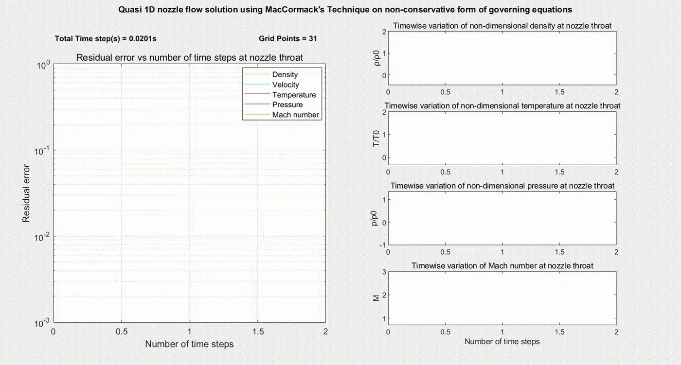
Fig. 3: Quasi 1D nozzle flow solution using MacCormack's technique on non-conservative form of governing equation for 31 grid points
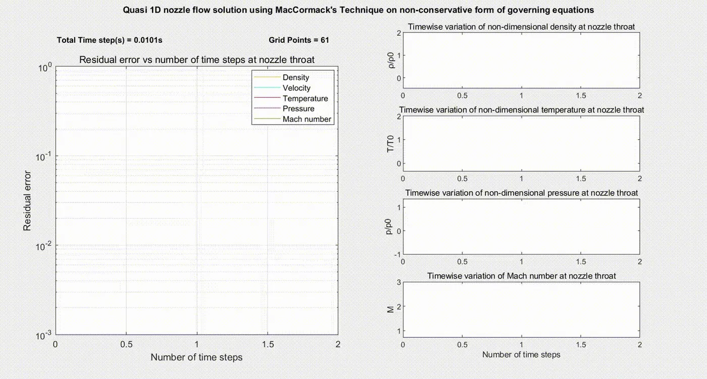
Fig. 4: Quasi 1D nozzle flow solution using MacCormack's technique on non-conservative form of governing equation for 61 grid points
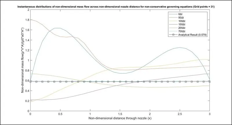
Fig. 5: Instantaneous distributions of non-dimensional mass flow across non-dimensional nozzle distance for non-conservative form of governing equations on 31 grid points domain
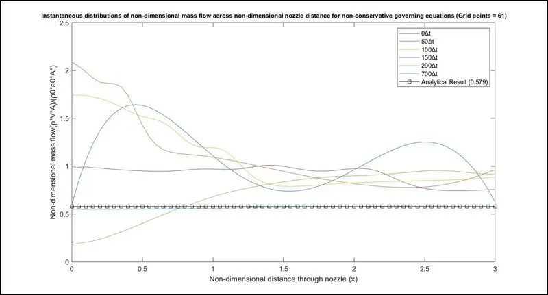
Fig. 6: Instantaneous distributions of non-dimensional mass flow across non-dimensional nozzle distance for non-conservative form of governing equations on 61 grid points domain
3.2 Computed values of non-dimensional primitive variables (density, temperature, pressure) and Mach number for the quasi 1D nozzle flow solution both in time and across non-dimensional distance through nozzle using MacCormack's method on conservative form of governing equations employed on grid size of 31 and 61 points
Fig. 7 and Fig. 8 below shows the timewise variations of non-dimensional primitive variables (density, temperature, pressure) and Mach number as well as residual error values computed for the same including for velocity using MacCormack's technique on the conservative form of governing equations for grid size of 31 and 61 points respectively. Similar to the previous subsection 3.1 under Section 3 Results, the residual error values were determined by computing the absolute difference for the aforementioned non-dimensional quantities at the nozzle throat area between the previous time step and current time step. The timewise variations for all of the concerned variables approach an almost steady state solution between the odd 600-800 time-steps mark region for grid size of 31 points and around the 900-1100 time-step mark for grid size of 61 points. This is also reiterated in Fig. 9 and Fig. 10 displaying the instantaneous distributions of non-dimensional mass flow across non-dimensional nozzle distance for the conservative form of governing equations employed on 31 and 61 grid points respectively, and here too it can be reasoned based on the values of time-step size evaluated with the former grid size predicting it to be 0.0204s while the latter grid size at 0.01018s respectively suggesting that more time steps are required before stability in outputs is observed as grid points increase across the domain. It should be noted that the time-step size value evaluated for the grid size of 31 points was anomalous to the same value reported in John D. Anderson, Jr., (1995), although the formulations for the same were consistent throughout with that described in John D. Anderson, Jr., (1995), and since no specific reason could be deduced, therefore the values should be considered with a small degree of caution despite them being nearly indistinguishable at smaller decimal positions. Interestingly, there are notable differences between the instantaneous distributions of the non-dimensional mass flow for both forms of governing equations wherein the variations are much less pronounced or rather less erratic for the conservative formulations as compared to the non-conservative ones.
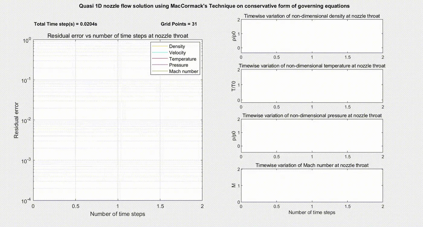
Fig. 7: Quasi 1D nozzle flow solution using MacCormack's technique on conservative form of governing equation for 31 grid points
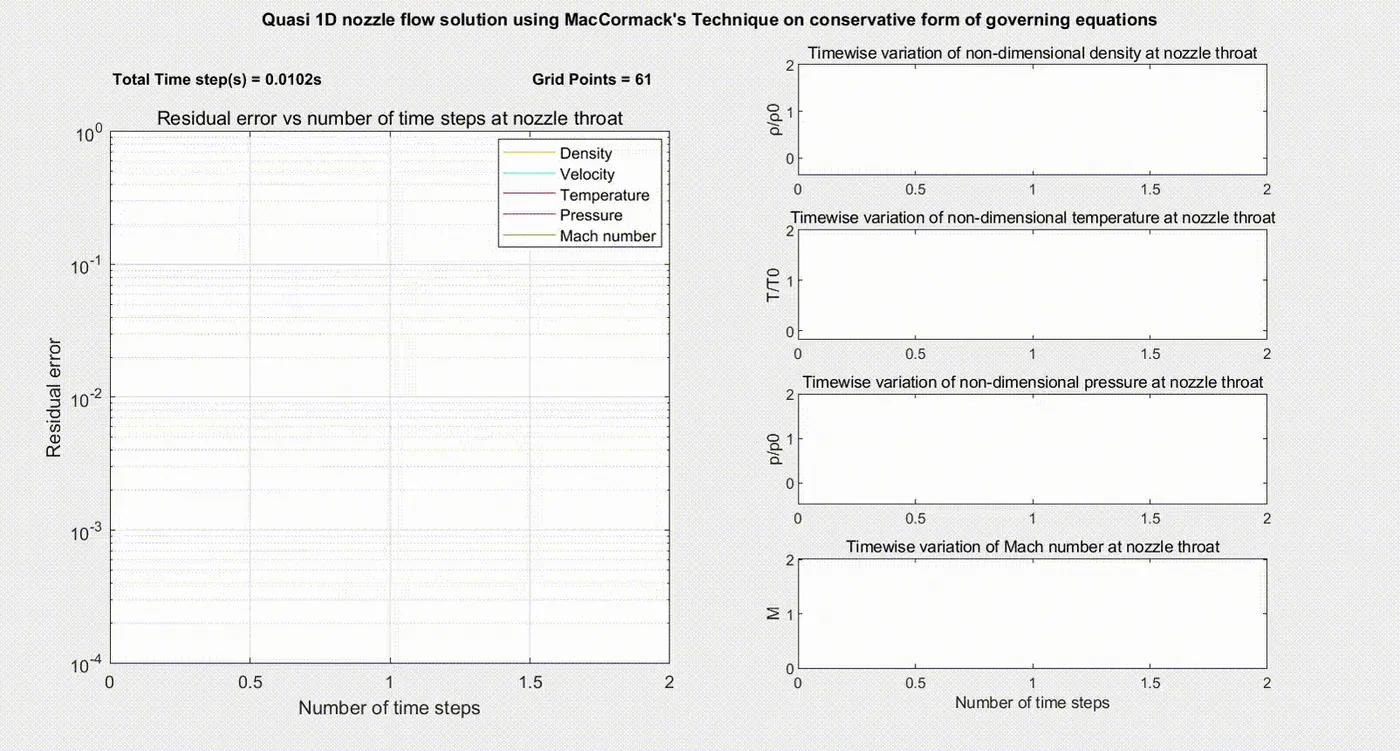
Fig. 8: Quasi 1D nozzle flow solution using MacCormack's technique on conservative form of governing equation for 61 grid points
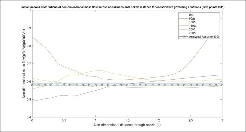
Fig. 9: Instantaneous distributions of non-dimensional mass flow across non-dimensional nozzle distance for conservative form of governing equations on 31 grid points domain
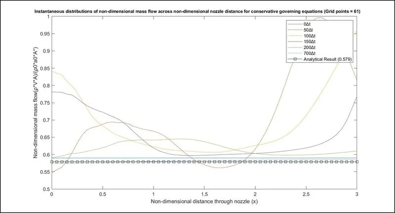
Fig. 10: Instantaneous distributions of non-dimensional mass flow across non-dimensional nozzle distance for conservative form of governing equations on 61 grid points domain
3.3 Comparison of steady-state distributions of non-dimensional primitive variables (density, temperature, pressure) and Mach number across non-dimensional distance through nozzle using MacCormack's method on both forms of governing equations for the quasi 1D nozzle flow solution between grid size of 31 and 61 points and exact analytical solution as well as non-dimensional mass flow between both forms of governing equations for mesh independent solution at 31 grid points and exact analytical solution
In Fig. 11 and Fig. 12, we can observe the differences in prediction of steady-state distributions of non-dimensional primitive variables and Mach number across the non-dimensional distance through nozzle for both conservative and non-conservative forms of governing equations with grid size of 31 and 61 points in comparison with the exact analytical solution. Based on the tabulated values of the same quantities of interest, mentioned previously, corresponding to the nozzle throat area it is signified that the variations are rather minimal at the cost of increasing grid points that subsequently increases number of time-steps towards achieving stable outputs at marginal values of improved accuracy by consequently decreasing the time-step size as has also been evident in the previous subsections under Section 3 Results with solutions for the grid sizes using both forms of governing equations showing an overall good agreement with the exact analytical solutions as displayed in the subplots of the corresponding variables. In other words, a grid independent result can be declared for the grid size of 31 points wherein the maximum variation observed was of 0.277% for the non-dimensional pressure variable with the non-conservative form of governing equations and 0.02546% for the same variable with the conservative form of governing equations across all non-dimensional variables and Mach number at the nozzle throat area. Fig. 13 below provides a comparison between the steady-state distributions of non-dimensional mass flow for both forms of governing equations at the end of the final time step of 1400 and it can be noticed that the conservative form of governing equations has an overall constant value that is much more in the vicinity of the exact analytical solution as opposed to the fluctuating value of the same variable with peaks towards either end of the nozzle distance for the non-conservative form of governing equations.
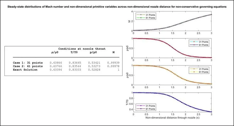
Fig. 11: Comparison of steady-state distributions of non-dimensional primitive variables and Mach number across non-dimensional distance through nozzle using MacCormack's method on non-conservative form of governing equations for the quasi 1D nozzle flow solution between grid size of 31 and 61 points and against exact analytical solution
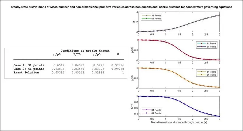
Fig. 12: Comparison of steady-state distributions of non-dimensional primitive variables and Mach number across non-dimensional distance through nozzle using MacCormack's method on conservative form of governing equations for the quasi 1D nozzle flow solution between grid size of 31 and 61 points and against exact analytical solution
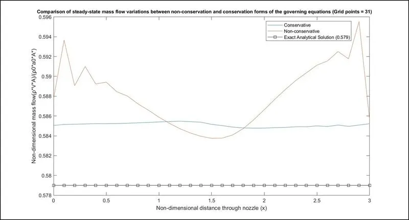
Fig. 13: Comparison of steady-state distributions of non-dimensional mass flow across non-dimensional distance through nozzle using MacCormack's method on both forms of governing equations for the quasi 1D nozzle flow solution at grid size of 31 points and against the exact analytical solution
4. Discussion
The distinctive comparisons between the two forms of governing equations when computed numerically for the quasi 1D nozzle flow solution using MacCormack's technique becomes significant on majorly the material points of initial conditions, principles that the two governing equations are based on i.e., conservative and non-conservative approaches, and behaviour of the residuals for the concerned variables. The role that the initial conditions play are of paramount importance with regards to the convergence of a numerical solution and the fact that the same defined for the conservative form of governing equations are more aligned with the realistic scenario on the account of the stability behaviour of the same as the formulations of the variables are more sensitive using this approach as opposed to the non-conservative form, the former form of governing equations perform better over the latter. This is also the case when initialising the non-dimensional mass flow quantity for the conservative form of governing equations which is assumed to be constant thereby ensuring mass is conserved throughout the computed flow field, apart from also being one of the dependent variables, and enabling an overall better agreement with the exact analytical solution on comparison with the formulation of the same quantity for the non-conservative form of governing equations. In regards to the residuals or the residual behaviour and despite both forms of the governing equations recording error values of a similar order at the initial time steps, it is the non-conservation form of governing equations that reaches a specified tolerance or convergence criterion, if there were one, before the conservative form of governing equations and this inherently comes down to the formulations leading to the inference that the non-conservative form of governing equations possessing a better "quality" of numerical algorithm over the conservative form. There are other factors also that affect the accuracy of a numerical solution using either form of governing equations including the "Inflow Boundary Condition error", "Truncation error in justification of grid independent results" and "Effects of Courant number" to name a few. The "Inflow Boundary Condition error" refers to the assumption that the values of primitive variables viz. density, pressure and temperature, resemble the reservoir conditions, however, this would only be true if the Mach number at the inflow boundary was to be equal to 0 which is not the case as the realistic inflow boundary condition has the area ratio as a finite value and as such the analytical and numerical solution would result in a finite numerical value of Mach number. Therefore, the numerical value of the non-dimensional density variable specified is 1 while the exact analytical solution results in 0.995 giving rise to a 0.5 percent error. "Truncation error in justification of grid independent results" points to the assumption that was made in identifying the grid independent solution for the given numerical problem wherein it was decided that the results obtained from number of grid points as 31 was at an acceptable level in comparison to the results from number of grid points as 61 even though the latter agreed better with the exact analytical solution based on the comparison between marginal difference in values over the increasing computational cost of time. Lastly, and in the context of the given numerical problem, "Effects of Courant number" does affect the stability of the numerical solution more so than the accuracy and although this was not investigated as the Courant number selected was 0.5, which is very much less than its limiting upper bound value of 1, the advantage that a higher Courant number offers is fewer time steps to reach a pre-determined non-dimensional time, which must be same when comparing different Courant numbers to observe differences, however with increasing concerns that at a particular time step and when the stability criterion is violated, the chances of the solution "blowing up" or to put it simply, begin to diverge from the intended actual solution also grows.
5. Conclusion
Solution for the quasi 1D nozzle flow numerical problem for both forms of governing equations using the MacCormack's technique in Matlab was well understood with this programming exercise. It was realised that based on similar assumptions of grid size, Courant number and subsequently the time-step evaluation, as well as appropriate initial and boundary conditions, the results obtained from either form of governing equations does not indicate any kind of superiority of any numerical algorithm. The calculation procedure and setup, however, proved to be a more time consuming effort for the conservative form over the non-conservative form of governing equations due to the additional decoding of primitive variables at the required stages of the solution. The implementation of the CFD methodologies for the given flow problem also highlighted the capabilities of performing and obtaining a numerical solution which agrees well with the exact analytical solutions and that this model can then be accordingly subjected to different flow problems of similar nature aiding in cost and material benefits during prototyping and other key areas of research and development, and manufacturing.
6. References
[1] John D. Anderson, Jr., (1995). COMPUTATIONAL FLUID DYNAMICS: The Basics with Applications (Eds.), Numerical Solutions of Quasi-One-Dimensional Nozzle Flows (2nd ed., pp. 283–356). McGraw-Hill.
[2] John D. Anderson, Jr., (2003). Modern Compressible Flow With Historical Perspective (Eds.), Quasi-One-Dimensional Flow (3rd ed., pp. 202–206). McGraw-Hill.
CODE:
Program to simulate the isentropic flow through a quasi 1D subsonic-supersonic nozzle using the MacCormack's technique on both the conservative and non-conservative forms of the governing equations.
clear all
close all
clc

%% Inputs for the quasi 1D nozzle flow simulation

% Domain Length

L = 3;

% Number of grid points along x direction in array form

n_x = [31,61];

% Ratio of specific heats (Cp/Cv) for air at standard conditions

gamma = 1.4;

%% Transient characteristics setup

% Number of time steps

time_steps = 1400;

% Courant number initialisation

Courant_number = 0.5;

%% Grid independence setup

% Number of grid independence variables comparison

grid_independence_variable_comparison = 6;

% Initialisation of different grid size arrays

[conservative_form_grid_1,non_conservative_form_grid_1] = deal(ones(grid_independence_variable_comparison,max(n_x)));

[rows,columns] = size(conservative_form_grid_1);

[conservative_form_grid_2,non_conservative_form_grid_2] = deal(ones(grid_independence_variable_comparison,max(n_x)));

%% Solution for conservative form of governing equations

% Creating arrays to store data corresponding to spatial grid size,
% density, temperature, pressure and Mach number values as well as an
% elements range array to access the same

conservative_form_grid_independence = vertcat(conservative_form_grid_1,conservative_form_grid_2);

elements_range = 1:size(conservative_form_grid_1);

Grid_Size = {sprintf('Case %d: %d points',1,n_x(1))};

[rho_grid_size,T_grid_size,p_grid_size,M_grid_size] = deal(1);

rho_grid_size_array = vertcat(rho_grid_size);

T_grid_size_array = vertcat(T_grid_size);

p_grid_size_array = vertcat(p_grid_size);

M_grid_size_array = vertcat(M_grid_size);

elements_range_array = horzcat(elements_range);

Grid_Size_array = vertcat(Grid_Size);

% Loop to define spatial grid size, nozzle shape A = A(x) which is fixed
% and independent of time, exact solutions for density, pressure and
% temperature based on the Area-Mach number relation and passing the
% required variables to calculate the variation of non-dimensional
% primitive variables i.e., density, temperature, and pressure across both
% non-dimensional nozzle distance and time steps as well as non-dimensional
% mass flow as a function of non-dimensional nozzle distance based on the
% conservative form of governing equations and dependent on the number of
% grid points

for grid_points = 1:length(n_x)

    if grid_points >= 2
        elements_range = (((grid_points-1)*rows)+1):(((grid_points-1)*rows)+(rows));
        Grid_Size = {sprintf('Case %d: %d points',grid_points,n_x(grid_points))};
        elements_range_array = horzcat(elements_range_array,elements_range);
        Grid_Size_array = vertcat(Grid_Size_array,Grid_Size);
    end

    % Function call to determine grid creation based on number of grid
    % points as well as setup of area profile

    [x, dx, A] = grid_initial_conditions_setup(L, n_x(grid_points));

    % Function call to evaluate the analytical/exact solution

    [M_exact, rho_exact, p_exact, T_exact] = exact_solution_mach_number_primitive_variables(x, A, gamma);

    % Analytical Mass flow value allocation

    non_dimensional_mass_flow_analytical(1,1:n_x(grid_points)) = 0.579;

    % Function call to compute non-dimensional mass flow and primitive
    % variables, and Mach Number based on conservative form of governing
    % equations

    [conservative_form_steady_state_mass_flow, rho, T, p, M] = Week_7_Quasi_1D_nozzle_flow_conservative(x, dx, n_x(grid_points), A, gamma, M_exact, rho_exact, p_exact, T_exact, time_steps, Courant_number);

    conservative_form_grid_independence(elements_range(1),1:n_x(grid_points)) = x;
    conservative_form_grid_independence(elements_range(2),1:n_x(grid_points)) = conservative_form_steady_state_mass_flow;
    conservative_form_grid_independence(elements_range(3),1:n_x(grid_points)) = rho;
    conservative_form_grid_independence(elements_range(4),1:n_x(grid_points)) = T;
    conservative_form_grid_independence(elements_range(5),1:n_x(grid_points)) = p;
    conservative_form_grid_independence(elements_range(6),1:n_x(grid_points)) = M;

    rho_grid_size = conservative_form_grid_independence(elements_range(3),1:n_x(grid_points));
    T_grid_size = conservative_form_grid_independence(elements_range(4),1:n_x(grid_points));
    p_grid_size = conservative_form_grid_independence(elements_range(5),1:n_x(grid_points));
    M_grid_size = conservative_form_grid_independence(elements_range(6),1:n_x(grid_points));
    rho_grid_size = rho_grid_size(A==1);
    T_grid_size = T_grid_size(A==1);
    p_grid_size = p_grid_size(A==1);
    M_grid_size = M_grid_size(A==1);
    rho_grid_size_array = vertcat(rho_grid_size_array,rho_grid_size);
    T_grid_size_array = vertcat(T_grid_size_array,T_grid_size);
    p_grid_size_array = vertcat(p_grid_size_array,p_grid_size);
    M_grid_size_array = vertcat(M_grid_size_array,M_grid_size);

end

% Creating a figure and defining its size based on positional limits

figure1 = figure('Position',[141,54,1070,575]);

% Defining title text for the entire plot

title_text_steady_state_distribution = sprintf("Steady-state distributions of Mach number and non-dimensional primitive variables across non-dimensional nozzle distance for conservative governing equations");
sgtitle(title_text_steady_state_distribution,'FontSize',9.5,'FontWeight','bold')

% Creating subplots within the main figure to initially plot the exact
% analytical solutions of non-dimensional primitive variables and Mach
% number followed by using their handles to update the same subplot with
% solutions obtained using the conservative form of governing equations for
% grid size of 31 and 61 points respectively

ax1 = subplot(4,2,2);
plot(x,M_exact,'color', [0 0 0], 'LineStyle', ':', 'HandleVisibility','off', 'LineWidth', 2)
ylabel('M');
hold on

ax2 = subplot(4,2,4);
plot(x,p_exact,'color', [0 0 0], 'LineStyle', ':', 'HandleVisibility','off', 'LineWidth', 2)
ylabel('p/p0');
hold on

ax3 = subplot(4,2,6);
plot(x,rho_exact,'color', [0 0 0], 'LineStyle', ':', 'HandleVisibility','off', 'LineWidth', 2)
ylabel('ρ/ρ0');
hold on

ax4 = subplot(4,2,8);
plot(x,T_exact,'color', [0 0 0], 'LineStyle', ':', 'HandleVisibility','off', 'LineWidth', 2)
ylabel('T/T0');
xlabel('Non-dimensional distance through nozzle (x)');
hold on

% Creating array with RGB Triplet values representing different plot line,
% and marker face and marker edge colours as well as the marker styles for
% ease in distinguishing

colour_mach_primitive_variables_comparison = [[0.4660 0.6740 0.1880];[0 1 1];[0.9290 0.6940 0.1250];[1 0 1];[0 1 0];[0 0 1];[1 1 0];[0.6350 0.0780 0.1840]];

marker_colour_mach_primitive_variables_comparison = [[0.49,0.18,0.56];[1.00,0.00,0.00];[0.85,0.33,0.10];[0.00,0.00,1.00]];

markers_mach_primitive_variables_comparison = {'-o';'-d'};

% Defining variables with initial values for navigating through different
% index positions of the concerned arrays in the forthcoming loop as well
% as initialising plot handles and plot labels that would store the name of
% the legend values

[j,l] = deal(1);

M_M_exact = zeros(1,length(n_x));
p_p_exact = zeros(1,length(n_x));
rho_rho_exact = zeros(1,length(n_x));
T_T_exact = zeros(1,length(n_x));

M_M_exactLabels = cell(1,length(n_x));
p_p_exactLabels = cell(1,length(n_x));
rho_rho_exactLabels = cell(1,length(n_x));
T_T_exactLabels = cell(1,length(n_x));

% Loop to plot the non-dimensional primitive variables and Mach number on
% top of their exact analytical solutions with the plot line, marker face
% and marker edge colours relating to the index position in their arrays

for i = 1:length(n_x)

        M_M_exact(i) = plot(ax1,conservative_form_grid_independence(((i-1)*rows)+1,1:n_x(i)),conservative_form_grid_independence(((i-1)*rows)+6,1:n_x(i)), char(markers_mach_primitive_variables_comparison(i)));
        set(M_M_exact(i), 'color', colour_mach_primitive_variables_comparison(j,:), 'LineWidth', 1, 'MarkerSize', 2, 'MarkerEdgeColor',marker_colour_mach_primitive_variables_comparison(l,:),'MarkerFaceColor',marker_colour_mach_primitive_variables_comparison(l,:));
        M_M_exactLabels{i} = [ num2str(n_x(i)) ' Points'];

        p_p_exact(i) = plot(ax2,conservative_form_grid_independence(((i-1)*rows)+1,1:n_x(i)),conservative_form_grid_independence(((i-1)*rows)+5,1:n_x(i)), char(markers_mach_primitive_variables_comparison(i)));
        set(p_p_exact(i), 'color', 	colour_mach_primitive_variables_comparison(j+1,:), 'LineWidth', 1, 'MarkerSize', 2, 'MarkerSize', 2, 'MarkerEdgeColor',marker_colour_mach_primitive_variables_comparison(l+1,:),'MarkerFaceColor',marker_colour_mach_primitive_variables_comparison(l+1,:));
        p_p_exactLabels{i} = [ num2str(n_x(i)) ' Points'];

        rho_rho_exact(i) = plot(ax3,conservative_form_grid_independence(((i-1)*rows)+1,1:n_x(i)),conservative_form_grid_independence(((i-1)*rows)+3,1:n_x(i)), char(markers_mach_primitive_variables_comparison(i)));
        set(rho_rho_exact(i), 'color', colour_mach_primitive_variables_comparison(j+2,:), 'LineWidth', 1, 'MarkerSize', 2, 'MarkerSize', 2, 'MarkerEdgeColor',marker_colour_mach_primitive_variables_comparison(l+2,:),'MarkerFaceColor',marker_colour_mach_primitive_variables_comparison(l+2,:));
        rho_rho_exactLabels{i} = [ num2str(n_x(i)) ' Points'];

        T_T_exact(i) = plot(ax4,conservative_form_grid_independence(((i-1)*rows)+1,1:n_x(i)),conservative_form_grid_independence(((i-1)*rows)+4,1:n_x(i)), char(markers_mach_primitive_variables_comparison(i)));
        set(T_T_exact(i), 'color', colour_mach_primitive_variables_comparison(j+3,:), 'LineWidth', 1, 'MarkerSize', 2, 'MarkerSize', 2, 'MarkerEdgeColor',marker_colour_mach_primitive_variables_comparison(l+3,:),'MarkerFaceColor',marker_colour_mach_primitive_variables_comparison(l+3,:));
        T_T_exactLabels{i} = [ num2str(n_x(i)) ' Points'];

        j = j+4;

end

% Plotting the legend with respect to the plot handles and plot labels

legend(M_M_exact,M_M_exactLabels,'Location','northwest')
legend(p_p_exact,p_p_exactLabels)
legend(rho_rho_exact,rho_rho_exactLabels)
legend(T_T_exact,T_T_exactLabels,'Location','southwest')

% Concatenating entries to pre-existing arrays

Grid_Size = {sprintf('Exact Solution')};

Grid_Size_array = vertcat(Grid_Size_array,Grid_Size);

rho_grid_size_array = vertcat(rho_grid_size_array,rho_exact(A==1));
T_grid_size_array = vertcat(T_grid_size_array,T_exact(A==1));
p_grid_size_array = vertcat(p_grid_size_array,p_exact(A==1));
M_grid_size_array = vertcat(M_grid_size_array,M_exact(A==1));

rho_grid_size_array(1) = [];
T_grid_size_array(1) = [];
p_grid_size_array(1) = [];
M_grid_size_array(1) = [];

% Defining a table to plot for comparison against different grid points
% indicating grid independence for values of non-dimensional primitive
% variables at the nozzle throat

grid_independence_conservative_table = table(rho_grid_size_array,T_grid_size_array,p_grid_size_array,M_grid_size_array,'RowNames',Grid_Size_array);
grid_independence_conservative_table.Properties.VariableNames = {'ρ/ρ0' 'T/T0' 'p/p0' 'M'};
grid_independence_conservative_table1 = table(grid_independence_conservative_table);
grid_independence_conservative_table1.Properties.VariableNames = {sprintf('                   Conditions at nozzle throat') };
grid_independence_conservative_table1_string = evalc('disp(grid_independence_conservative_table1)');

% Using TeX Markup to define bold formatting along with underscores

grid_independence_conservative_table1_string = strrep(grid_independence_conservative_table1_string,'','bf');
grid_independence_conservative_table1_string = strrep(grid_independence_conservative_table1_string,'','rm');
grid_independence_conservative_table1_string = strrep(grid_independence_conservative_table1_string,'_','_');

% Creating fixed-width font

FixedWidth = get(0,'FixedWidthFontName');

% Creating table in the same figure using the annotation function

annotation(gcf,'Textbox','String',grid_independence_conservative_table1_string,'Interpreter','Tex','FontName',FixedWidth,'Units','Normalized','Position',[0.0180 0.398 0.505 0.236])

% Save plot of steady state distributions of non-dimensional primitive
% variable and Mach number using the conservative form of governing
% equations for grid size of 31 and 61 points respectively as a function of
% the non-dimensional distance through nozzle

saveas(figure1,sprintf('Steady_state_distributions_Mach_Number_non_dimensional_primitive_variables_conservative.jpg'));
close(figure1);

%% Solution for non-conservative form of governing equations

% Creating arrays to store data corresponding to spatial grid size,
% density, temperature, pressure and Mach number values as well as an
% elements range array to access the same

non_conservative_form_grid_independence = vertcat(non_conservative_form_grid_1,non_conservative_form_grid_2);

elements_range = 1:size(non_conservative_form_grid_1);

Grid_Size = {sprintf('Case %d: %d points',1,n_x(1))};

[rho_grid_size,T_grid_size,p_grid_size,M_grid_size] = deal(1);

rho_grid_size_array = vertcat(rho_grid_size);

T_grid_size_array = vertcat(rho_grid_size);

p_grid_size_array = vertcat(rho_grid_size);

M_grid_size_array = vertcat(rho_grid_size);

elements_range_array = horzcat(elements_range);

Grid_Size_array = vertcat(Grid_Size);

% Loop to define spatial grid size, nozzle shape A = A(x) which is fixed
% and independent of time, exact solutions for density, pressure and
% temperature based on the Area-Mach number relation and passing the
% required variables to calculate the variation of non-dimensional
% primitive variables i.e., density, temperature, and pressure across both
% non-dimensional nozzle distance and time steps as well as non-dimensional
% mass flow as a function of non-dimensional nozzle distance based on the
% non-conservative form of governing equations and dependent on the number
% of grid points

for grid_points = 1:length(n_x)

    if grid_points >= 2
        elements_range = (((grid_points-1)*rows)+1):(((grid_points-1)*rows)+(rows));
        Grid_Size = {sprintf('Case %d: %d points',grid_points,n_x(grid_points))};
        elements_range_array = horzcat(elements_range_array,elements_range);
        Grid_Size_array = vertcat(Grid_Size_array,Grid_Size);
    end

    % Function call to determine grid creation based on number of grid
    % points as well as setup of area profile

    [x, dx, A] = grid_initial_conditions_setup(L, n_x(grid_points));

    % Function call to evaluate the analytical/exact solution

    [M_exact, rho_exact, p_exact, T_exact] = exact_solution_mach_number_primitive_variables(x, A, gamma);

    % Analytical Mass flow value allocation

    non_dimensional_mass_flow_analytical(1,1:n_x(grid_points)) = 0.579;

    % Function call to compute non-dimensional mass flow and primitive
    % variables, and Mach Number based on non-conservative form of
    % governing equations

    [non_conservative_form_steady_state_mass_flow, rho, T, p, M] = Week_7_Quasi_1D_nozzle_flow_non_conservative(x, dx, n_x(grid_points), A, gamma, M_exact, rho_exact, p_exact, T_exact, time_steps, Courant_number);
    non_conservative_form_grid_independence(elements_range(1),1:n_x(grid_points)) = x;
    non_conservative_form_grid_independence(elements_range(2),1:n_x(grid_points)) = non_conservative_form_steady_state_mass_flow;
    non_conservative_form_grid_independence(elements_range(3),1:n_x(grid_points)) = rho;
    non_conservative_form_grid_independence(elements_range(4),1:n_x(grid_points)) = T;
    non_conservative_form_grid_independence(elements_range(5),1:n_x(grid_points)) = p;
    non_conservative_form_grid_independence(elements_range(6),1:n_x(grid_points)) = M;

    rho_grid_size = non_conservative_form_grid_independence(elements_range(3),1:n_x(grid_points));
    T_grid_size = non_conservative_form_grid_independence(elements_range(4),1:n_x(grid_points));
    p_grid_size = non_conservative_form_grid_independence(elements_range(5),1:n_x(grid_points));
    M_grid_size = non_conservative_form_grid_independence(elements_range(6),1:n_x(grid_points));
    rho_grid_size = rho_grid_size(A==1);
    T_grid_size = T_grid_size(A==1);
    p_grid_size = p_grid_size(A==1);
    M_grid_size = M_grid_size(A==1);
    rho_grid_size_array = vertcat(rho_grid_size_array,rho_grid_size);
    T_grid_size_array = vertcat(T_grid_size_array,T_grid_size);
    p_grid_size_array = vertcat(p_grid_size_array,p_grid_size);
    M_grid_size_array = vertcat(M_grid_size_array,M_grid_size);

end

% Creating a figure and defining its size based on positional limits

figure2 = figure('Position',[141,54,1070,575]);

% Defining title text for the entire plot

title_text_steady_state_distribution = sprintf("Steady-state distributions of Mach number and non-dimensional primitive variables across non-dimensional nozzle distance for non-conservative governing equations");
sgtitle(title_text_steady_state_distribution,'FontSize',9.5,'FontWeight','bold')

% Creating subplots within the main figure to initially plot the exact
% analytical solutions of non-dimensional primitive variables and Mach
% number followed by using their handles to update the same subplot with
% solutions obtained using the non-conservative form of governing equations
% for grid size of 31 and 61 points respectively

ax1 = subplot(4,2,2);
plot(x,M_exact,'color', [0 0 0], 'LineStyle', ':', 'HandleVisibility','off', 'LineWidth', 2)
ylabel('M');
hold on

ax2 = subplot(4,2,4);
plot(x,p_exact,'color', [0 0 0], 'LineStyle', ':', 'HandleVisibility','off', 'LineWidth', 2)
ylabel('p/p0');
hold on

ax3 = subplot(4,2,6);
plot(x,rho_exact,'color', [0 0 0], 'LineStyle', ':', 'HandleVisibility','off', 'LineWidth', 2)
ylabel('ρ/ρ0');
hold on

ax4 = subplot(4,2,8);
plot(x,T_exact,'color', [0 0 0], 'LineStyle', ':', 'HandleVisibility','off', 'LineWidth', 2)
ylabel('T/T0');
xlabel('Non-dimensional distance through nozzle (x)');
hold on

% Creating array with RGB Triplet values representing different plot line,
% and marker face and marker edge colours as well as the marker styles for
% ease in distinguishing

[j,l] = deal(1);

M_M_exact = zeros(1,length(n_x));
p_p_exact = zeros(1,length(n_x));
rho_rho_exact = zeros(1,length(n_x));
T_T_exact = zeros(1,length(n_x));

M_M_exactLabels = cell(1,length(n_x));
p_p_exactLabels = cell(1,length(n_x));
rho_rho_exactLabels = cell(1,length(n_x));
T_T_exactLabels = cell(1,length(n_x));

% Loop to plot the non-dimensional primitive variables and Mach number on
% top of their exact analytical solutions with the plot line, marker face
% and marker edge colours relating to the index position in their arrays

for i = 1:length(n_x)

        M_M_exact(i) = plot(ax1,non_conservative_form_grid_independence(((i-1)*rows)+1,1:n_x(i)),non_conservative_form_grid_independence(((i-1)*rows)+6,1:n_x(i)), char(markers_mach_primitive_variables_comparison(i)));
        set(M_M_exact(i), 'color', colour_mach_primitive_variables_comparison(j,:), 'LineWidth', 1, 'MarkerSize', 2, 'MarkerEdgeColor',marker_colour_mach_primitive_variables_comparison(l,:),'MarkerFaceColor',marker_colour_mach_primitive_variables_comparison(l,:));
        M_M_exactLabels{i} = [ num2str(n_x(i)) ' Points'];

        p_p_exact(i) = plot(ax2,non_conservative_form_grid_independence(((i-1)*rows)+1,1:n_x(i)),non_conservative_form_grid_independence(((i-1)*rows)+5,1:n_x(i)), char(markers_mach_primitive_variables_comparison(i)));
        set(p_p_exact(i), 'color', 	colour_mach_primitive_variables_comparison(j+1,:), 'LineWidth', 1, 'MarkerSize', 2, 'MarkerSize', 2, 'MarkerEdgeColor',marker_colour_mach_primitive_variables_comparison(l+1,:),'MarkerFaceColor',marker_colour_mach_primitive_variables_comparison(l+1,:));
        p_p_exactLabels{i} = [ num2str(n_x(i)) ' Points'];

        rho_rho_exact(i) = plot(ax3,non_conservative_form_grid_independence(((i-1)*rows)+1,1:n_x(i)),non_conservative_form_grid_independence(((i-1)*rows)+3,1:n_x(i)), char(markers_mach_primitive_variables_comparison(i)));
        set(rho_rho_exact(i), 'color', colour_mach_primitive_variables_comparison(j+2,:), 'LineWidth', 1, 'MarkerSize', 2, 'MarkerSize', 2, 'MarkerEdgeColor',marker_colour_mach_primitive_variables_comparison(l+2,:),'MarkerFaceColor',marker_colour_mach_primitive_variables_comparison(l+2,:));
        rho_rho_exactLabels{i} = [ num2str(n_x(i)) ' Points'];

        T_T_exact(i) = plot(ax4,non_conservative_form_grid_independence(((i-1)*rows)+1,1:n_x(i)),non_conservative_form_grid_independence(((i-1)*rows)+4,1:n_x(i)), char(markers_mach_primitive_variables_comparison(i)));
        set(T_T_exact(i), 'color', colour_mach_primitive_variables_comparison(j+3,:), 'LineWidth', 1, 'MarkerSize', 2, 'MarkerSize', 2, 'MarkerEdgeColor',marker_colour_mach_primitive_variables_comparison(l+3,:),'MarkerFaceColor',marker_colour_mach_primitive_variables_comparison(l+3,:));
        T_T_exactLabels{i} = [ num2str(n_x(i)) ' Points'];

        j = j+4;

end

% Plotting the legend with respect to the plot handles and plot labels

legend(M_M_exact,M_M_exactLabels,'Location','northwest')
legend(p_p_exact,p_p_exactLabels)
legend(rho_rho_exact,rho_rho_exactLabels)
legend(T_T_exact,T_T_exactLabels,'Location','southwest')

% Concatenating entries to pre-existing arrays

Grid_Size = {sprintf('Exact Solution')};

Grid_Size_array = vertcat(Grid_Size_array,Grid_Size);

rho_grid_size_array = vertcat(rho_grid_size_array,rho_exact(A==1));
T_grid_size_array = vertcat(T_grid_size_array,T_exact(A==1));
p_grid_size_array = vertcat(p_grid_size_array,p_exact(A==1));
M_grid_size_array = vertcat(M_grid_size_array,M_exact(A==1));

rho_grid_size_array(1) = [];
T_grid_size_array(1) = [];
p_grid_size_array(1) = [];
M_grid_size_array(1) = [];

% Defining a table to plot for comparison against different grid points
% indicating grid independence for values of non-dimensional primitive
% variables at the nozzle throat

grid_independence_non_conservative_table = table(rho_grid_size_array,T_grid_size_array,p_grid_size_array,M_grid_size_array,'RowNames',Grid_Size_array);
grid_independence_non_conservative_table.Properties.VariableNames = {'ρ/ρ0' 'T/T0' 'p/p0' 'M'};
grid_independence_non_conservative_table1 = table(grid_independence_non_conservative_table);
grid_independence_non_conservative_table1.Properties.VariableNames = {sprintf('                   Conditions at nozzle throat') };
grid_independence_non_conservative_table1_string = evalc('disp(grid_independence_non_conservative_table1)');

% Using TeX Markup to define bold formatting along with underscores

grid_independence_non_conservative_table1_string = strrep(grid_independence_non_conservative_table1_string,'','bf');
grid_independence_non_conservative_table1_string = strrep(grid_independence_non_conservative_table1_string,'','rm');
grid_independence_non_conservative_table1_string = strrep(grid_independence_non_conservative_table1_string,'_','_');

% Creating fixed-width font

FixedWidth = get(0,'FixedWidthFontName');

% Creating table in the same figure using the annotation function

annotation(gcf,'Textbox','String',grid_independence_non_conservative_table1_string,'Interpreter','Tex','FontName',FixedWidth,'Units','Normalized','Position',[0.0180 0.398 0.505 0.236])

% Save plot of steady state distributions of non-dimensional primitive
% variable and Mach number using the non-conservative form of governing
% equations for grid size of 31 and 61 points respectively as a function of
% the non-dimensional distance through nozzle

saveas(figure2,sprintf('Steady_state_distributions_Mach_Number_non_dimensional_primitive_variables_non_conservative.jpg'));
close(figure2);

%% Combined Plots

% Creating a figure and defining its size based on positional limits

figure3 = figure('Position',[141,54,1070,575]);

% Reinitialising the elements range array to navigate through solutions
% obtained from grid independent results

elements_range = 1:size(non_conservative_form_grid_1);

% Analytical Mass flow value allocation based on grid independent size

non_dimensional_mass_flow_analytical(1,1:n_x(1)) = 0.579;

% Plot of non-dimensional mass flow as a function of non-dimensional
% distance through nozzle at the final time step of 1400 using both
% conservative and non-conservative form of governing equations as well as
% the exact analytical solution based on the grid independent results

plot(conservative_form_grid_independence(elements_range(1),1:n_x(1)),conservative_form_grid_independence(elements_range(2),1:n_x(1)))
hold on
plot(non_conservative_form_grid_independence(elements_range(1),1:n_x(1)),non_conservative_form_grid_independence(elements_range(2),1:n_x(1)))
plot(conservative_form_grid_independence(elements_range(1),1:n_x(1)),non_dimensional_mass_flow_analytical(1,1:n_x(1)),'k-s')
ylabel('Non-dimensional mass flow(ρ*V*A)/(ρ0*a0*A*)');
xlabel('Non-dimensional distance through nozzle (x)');
legend_text_conservative = sprintf('Conservative');
legend_text_non_conservative = sprintf('Non-conservative');
legend_text_exact_analytical_solution = sprintf('Exact Analytical Solution (%.3f)',non_dimensional_mass_flow_analytical(1));
Lgnd = legend(legend_text_conservative,legend_text_non_conservative,legend_text_exact_analytical_solution);
set(Lgnd,'Position',[0.671 0.817 0.169 0.0886])
sgtitle(sprintf('Comparison of steady-state mass flow variations between non-conservation and conservation forms of the governing equations (Grid points = %d)',n_x(1)),'FontSize',9.5,'FontWeight','bold')

% Save plot of non-dimensional mass flow as a function of non-dimensional
% distance through nozzle at the final time step of 1400 using both
% conservative and non-conservative form of governing equations as well as
% the exact analytical solution based on the grid independent results

saveas(figure3,sprintf('Comparison_steady_state_mass_flow_non_conservative_conservative_forms_governing_equations.jpg'));
% close(figure3);

%% Function for grid creation and setup of area profile

function [x, dx, A] = grid_initial_conditions_setup(L, n_x)

    % Creating mesh using linspace command

    x = linspace(0,L,n_x);

    % Defining the smallest length element of the domain

    dx = x(2)-x(1);

    % Evaluating area profile, A = A(x), which is fixed and independent of
    % time in the form of parabolic distribution

    A = 1+2.2*(x-1.5).^2;

end

%% Function for evaluating exact analytical solution of non-dimensional primitive variables based on Area-Mach number relation

function [M_exact, rho_exact, p_exact, T_exact] = exact_solution_mach_number_primitive_variables(x, A, gamma)

    % Mach number

    M_exact = deal(ones(size(x)));

    for M_exact_sol = 1:length(M_exact)
        syms M_exact_2
        assume(M_exact_2,'real')

        % Calculation of subsonic root i.e., M<1

        if M_exact_sol<=find(A==1)
            M_subsonic_root = vpasolve(((1/M_exact_2^2)*((2/(gamma+1))*(1+((gamma-1)/2)*M_exact_2^2))^((gamma+1)/(gamma-1)))-A(M_exact_sol)^2 == 0, M_exact_2, [1e-6 1+1e-12]);
            if (all(M_subsonic_root == M_subsonic_root(1)))
                M_subsonic_root = M_subsonic_root(1);
            end
            M_exact(M_exact_sol) = M_subsonic_root;

        % Calculation of supersonic root i.e., M>1

        else
            M_supersonic_root = vpasolve(((1/M_exact_2^2)*((2/(gamma+1))*(1+((gamma-1)/2)*M_exact_2^2))^((gamma+1)/(gamma-1)))-A(M_exact_sol)^2 == 0, M_exact_2, [1+1e-6 10]);
            if (all(M_supersonic_root == M_supersonic_root(1)))
                M_supersonic_root = M_supersonic_root(1);
            end
            M_exact(M_exact_sol) = M_supersonic_root;
        end
    end

    % Density

    rho_exact = (1+(((gamma-1)/2).*M_exact.^2)).^(-1/(gamma-1));

    % Pressure

    p_exact = (1+(((gamma-1)/2).*M_exact.^2)).^(-gamma/(gamma-1));

    % Temperature

    T_exact = (1+(((gamma-1)/2).*M_exact.^2)).^(-1);

end
Week_7_Quasi_1D_nozzle_flow_conservative function to simulate the isentropic flow through a quasi 1D subsonic-supersonic nozzle using the MacCormack's technique on the conservative form of governing equations
% Week_7_Quasi_1D_nozzle_flow_conservative to calculate quasi 1D nozzle
% flow solution based on conservative form of governing equations

function [conservative_form_steady_state_mass_flow, rho, T, p, M] = Week_7_Quasi_1D_nozzle_flow_conservative(x, dx, n_x, A, gamma, M_exact, rho_exact, p_exact, T_exact, time_steps, Courant_number)

% Initialising error values for non-dimensional primitive variables and
% Mach number

[error_rho,error_V,error_T,error_M,error_p] = deal(9e9);

% Initialising non-dimensional primitive variables of density and
% temperature followed by determining their initial profiles/initial
% conditions based on different intervals along the non-dimensional
% distance through nozzle

[rho,T] = deal(ones(size(x)));

for initial_conditions = 1:length(x)
    if  x(initial_conditions)>=0 && x(initial_conditions)<=0.5
        rho(initial_conditions) = 1;
        T(initial_conditions) = 1;
    elseif x(initial_conditions)>=0.5 && x(initial_conditions)<= 1.5
        rho(initial_conditions) = 1-0.366*(x(initial_conditions)-0.5);
        T(initial_conditions) = 1-0.167*(x(initial_conditions)-0.5);
    elseif x(initial_conditions)>=1.5 && x(initial_conditions)<= 3.5
        rho(initial_conditions) = 0.634-0.3879*(x(initial_conditions)-1.5);
        T(initial_conditions) = 0.833-0.3507*(x(initial_conditions)-1.5);
    end
end

% Calculating the initial profile of non-dimensional velocity variable
% based on the values of non-dimensional density variable and area profile
% relating to the corresponding grid size

V = 0.59./(rho.*A);

% Initialising non-dimensional pressure variable profile and Mach number
% based on the grid size

[p,M] = deal(ones(size(x)));

% Initialising solutions vectors

U1 = rho.*A;
U2 = rho.*A.*V;
U3 = rho.*((T./(gamma-1))+(gamma/2).*V.^2).*A;

% Evaluating flux vectors from the initialised solutions vector

F1 = U2;
F2 = ((U2.^2./U1)+(((gamma-1)/gamma).*(U3 - ((gamma/2)*(U2.^2./U1)))));
F3 = (((gamma.*U2.*U3)./U1)-((((gamma*(gamma-1))/2))*((U2.^3)./U1.^2)));

% Initialising source term vector

J2 = ones(1,n_x-1);

% Allocating non-dimensional primitive variables and mass flow to their
% respective arrays based on the value of non-dimensional primitive
% variables and mass flow at the nozzle throat

non_dimensional_density_throat(1,1) = rho(A==1);
non_dimensional_pressure_throat(1,1) = p(A==1);
non_dimensional_temperature_throat(1,1) = T(A==1);
non_dimensional_mach_number_throat(1,1) = M(A==1);
non_dimensional_mass_flow = ones(6,n_x);
non_dimensional_mass_flow_time_steps = ones(1,6);
non_dimensional_mass_flow_analytical(1,1:n_x) = 0.579;
non_dimensional_mass_flow(1,:) = rho.*V.*A;
non_dimensional_mass_flow_time_steps(1) = 0;

% Creating error arrays to store error values during the time-marching
% solution

error_update_rho(1,1) = error_rho;
error_update_V(1,1) = error_V;
error_update_T(1,1) = error_T;
error_update_M(1,1) = error_M;
error_update_p(1,1) = error_p;

% Evaluation of time step size

dt = min(Courant_number*(dx./(V+(T.^(0.5)))));

% Creating a figure and defining its size based on positional limits

figure1 = figure('Position',[141,54,1070,575]);

% Creating textbox with initial values of total time step(s) [in s] and
% grid points inside the figure at pre-determined positional limits
% as well as title of the plot

str_title_text = strcat(sprintf("Quasi 1D nozzle flow solution using MacCormack's Technique on conservative form of governing equations"));

str_time_step = strcat('Total Time step = ',{' '},num2str(dt),'s');

str_grid_points = strcat('Grid Points = ',{' '},num2str(n_x));

text_box_title_text = annotation('textbox', [0.055,0.950,0.904,0.0475], ...
            'String', str_title_text, ...
            'EdgeColor', 'none', ...
            'HorizontalAlignment', 'center','VerticalAlignment', 'top', ...
            'FitBoxToText','on');
            text_box_title_text.FontSize = 10;
            text_box_title_text.FontWeight = 'bold';

text_box_time_step = annotation('textbox', [0.0706,0.872,0.169,0.044], ...
            'String', str_time_step, ...
            'EdgeColor', 'none', ...
            'HorizontalAlignment', 'center', ...
            'FitBoxToText','on');
            text_box_time_step.FontSize = 9;
            text_box_time_step.FontWeight = 'bold';

text_box_grid_points = annotation('textbox', [0.3688 0.872 0.109 0.044], ...
            'String', str_grid_points, ...
            'EdgeColor', 'none', ...
            'HorizontalAlignment', 'center', ...
            'FitBoxToText','on');
            text_box_grid_points.FontSize = 9;
            text_box_grid_points.FontWeight = 'bold';

% Creating an animation file of format type .avi

animation_file_name = strcat(sprintf('Quasi_1D_nozzle_flow_MacCormack_Technique_conservative_grid_size_%d',n_x),'.avi');

obj = VideoWriter(animation_file_name);
obj.Quality = 100;
obj.FrameRate = 20;
obj.open();

% Time-Marching Solution

for k = 1:time_steps

    % Updating current time step values of different non-dimensional
    % primitive variables and Mach number to previous time step for
    % arriving in order to arrive at converged solution as well as to
    % compare the values of residual error

    U1_old = U1;
    U2_old = U2;
    U3_old = U3;
    rho_old = rho;
    V_old = V;
    T_old = T;
    p_old = p;
    M_old = M;

    % Predictor step
    % Initialising predictor arrays for solutions and source term vectors

    U1_time_derivative_predictor = ones(1,n_x-1);
    U2_time_derivative_predictor = ones(1,n_x-1);
    U3_time_derivative_predictor = ones(1,n_x-1);
    J2(1) = (1/gamma)*rho(1)*T(1)*(A(1)/dx);
    J2(end) = (1/gamma)*rho(end)*T(end)*(A(end)/dx);

    % Space loop using Forward differencing scheme

    for j=2:n_x-1

        A_spatial_derivative = (A(j+1)-A(j))/dx;
        J2(j) = (1/gamma)*rho(j)*T(j)*A_spatial_derivative;
        U1_time_derivative_predictor(j) = (-(F1(j+1)-F1(j)))/dx;
        U2_time_derivative_predictor(j) = -((F2(j+1)-F2(j))/dx)+J2(j);
        U3_time_derivative_predictor(j) = -((F3(j+1)-F3(j))/dx);

        % Solution Update of solutions vectors

        U1(j) = U1(j)+(U1_time_derivative_predictor(j)*dt);
        U2(j) = U2(j)+(U2_time_derivative_predictor(j)*dt);
        U3(j) = U3(j)+(U3_time_derivative_predictor(j)*dt);

    end

    % Initialising Boundary Conditions at Inlet for the solutions vectors

    U1(1) = rho(1)*A(1);
    U2(1) = (2*U2(2))-U2(3);
    U3(1) = U1(1)*((T(1)/(gamma-1))+(gamma/2)*(V(1)^2));

    % Decoding primitive variables from solutions vectors

    rho = U1./A;
    T = (gamma-1)*((U3./U1)-((gamma/2)*(U2./U1).^2));

    % Updating flux vectors for the corrector step

    F1 = U2;
    F2 = (((U2.^2)./U1)+(((gamma-1)/gamma).*(U3 - ((gamma/2)*((U2.^2)./U1)))));
    F3 = (((gamma.*U2.*U3)./U1)-((((gamma*(gamma-1))/2))*((U2.^3)./U1.^2)));

    % Corrector step
    % Initialising corrector arrays for solutions and source term vectors

    U1_time_derivative_corrector = ones(1,n_x-1);
    U2_time_derivative_corrector = ones(1,n_x-1);
    U3_time_derivative_corrector = ones(1,n_x-1);
    J2(1)= (1/gamma)*rho(1)*T(1)*(A(1)/dx);
    J2(end) = (1/gamma)*rho(end)*T(end)*(A(end)/dx);

    % Space loop using Backward differencing scheme

    for j=2:n_x-1

        A_spatial_derivative = (A(j)-A(j-1))/dx;
        J2(j) = (1/gamma)*rho(j)*T(j)*A_spatial_derivative;
        U1_time_derivative_corrector(j) = -(F1(j)-F1(j-1))/dx;
        U2_time_derivative_corrector(j) = (-((F2(j)-F2(j-1)))/dx)+J2(j);
        U3_time_derivative_corrector(j) = -((F3(j)-F3(j-1))/dx);

    end

    % Compute average derivatives for solutions vectors time derivatives

    U1_time_derivative = 0.5*(U1_time_derivative_predictor+U1_time_derivative_corrector);
    U2_time_derivative = 0.5*(U2_time_derivative_predictor+U2_time_derivative_corrector);
    U3_time_derivative = 0.5*(U3_time_derivative_predictor+U3_time_derivative_corrector);

    % Solution update of solutions vectors

    for i=2:n_x-1
        U1(i) = U1_old(i) + U1_time_derivative(i)*dt;
        U2(i) = U2_old(i) + U2_time_derivative(i)*dt;
        U3(i) = U3_old(i) + U3_time_derivative(i)*dt;
    end

    % Initialising Boundary Conditions at Outlet for the solutions vectors

    U1(n_x) = 2*U1(n_x-1)-U1(n_x-2);
    U2(n_x) = 2*U2(n_x-1)-U2(n_x-2);
    U3(n_x) = 2*U3(n_x-1)-U3(n_x-2);

    % Decoding primitive variables from solutions vectors

    rho = U1./A;
    V = U2./U1;
    T = (gamma-1)*((U3./U1)-((gamma/2).*(V.^2)));

    % Updating non-dimensional pressure variable and Mach number values
    % based on decoded primitive variables from solutions vectors

    p = rho.*T;
    M = V./T.^(1/2);

    % Updating flux vectors before being reused in the predictor step of
    % the next time step

    F1 = U2;
    F2 = (((U2.^2)./U1)+(((gamma-1)/gamma).*(U3 - ((gamma/2)*((U2.^2)./U1)))));
    F3 = (((gamma.*U2.*U3)./U1)-((((gamma*(gamma-1))/2))*((U2.^3)./U1.^2)));

    % Allocating the non-dimensional primitive variables and Mach number
    % values at the nozzle throat to their corresponding arrays at the
    % current time step

    non_dimensional_density_throat(1,k) = rho(A==1);
    non_dimensional_pressure_throat(1,k) = p(A==1);
    non_dimensional_temperature_throat(1,k) = T(A==1);
    non_dimensional_mach_number_throat(1,k) = M(A==1);

    % Storing the non-dimensional mass flow values at different time steps
    % during the time-marching solution

    if k==50
        non_dimensional_mass_flow(2,:) = rho.*V.*A;
        non_dimensional_mass_flow_time_steps(2) = k;
    elseif k==100
        non_dimensional_mass_flow(3,:) = rho.*V.*A;
        non_dimensional_mass_flow_time_steps(3) = k;
    elseif k==150
        non_dimensional_mass_flow(4,:) = rho.*V.*A;
        non_dimensional_mass_flow_time_steps(4) = k;
    elseif k==200
        non_dimensional_mass_flow(5,:) = rho.*V.*A;
        non_dimensional_mass_flow_time_steps(5) = k;
    elseif k==700
        non_dimensional_mass_flow(6,:) = rho.*V.*A;
        non_dimensional_mass_flow_time_steps(6) = k;
    end

    % Updating the time step number value to its corresponding array

    time_step_number_unsteady_state_explicit_array = 1:k;

    % Evaluating the absolute error values between the current time step
    % and previous time step for non-dimensional primitive variables
    % and Mach number

    error_rho = abs(rho_old(A==1)-rho(A==1));
    error_update_rho(1,k) = error_rho;
    error_V = abs(V_old(A==1)-V(A==1));
    error_update_V(1,k) = error_V;
    error_T = abs(T_old(A==1)-T(A==1));
    error_update_T(1,k) = error_T;
    error_M = abs(M_old(A==1)-M(A==1));
    error_update_M(1,k) = error_M;
    error_p = abs(p_old(A==1)-p(A==1));
    error_update_p(1,k) = error_p;

    % Condition to exit time-marching loop if error values are reported as
    % NaN or exceed a value of greater than 1e4

    if (isnan(error_rho)|isnan(error_V)|isnan(error_T)|isnan(error_M)|isnan(error_p))==1
       break;
    elseif (error_rho|error_V|error_T|error_M|error_p)>1e4
        break;
    end

    % Updating the Total Time step(s) during the time-marching loop

    text_box_time_step.String = sprintf("Total Time step(s) = %.4fs",dt*k);

    % Creating subplots within the main figure to plot the time-wise
    % variation of non-dimensional primitive variables and Mach
    % number as well as their respective error values during the
    % time-marching loop

    subplot(4,2,2)
    plot(time_step_number_unsteady_state_explicit_array,non_dimensional_density_throat,'k');
    title(sprintf("Timewise variation of non-dimensional density at nozzle throat"),'FontWeight','normal')
    ylabel('ρ/ρ0');

    subplot(4,2,4)
    plot(time_step_number_unsteady_state_explicit_array,non_dimensional_temperature_throat,'k');
    title(sprintf("Timewise variation of non-dimensional temperature at nozzle throat"),'FontWeight','normal')
    ylabel('T/T0');

    subplot(4,2,6)
    plot(time_step_number_unsteady_state_explicit_array,non_dimensional_pressure_throat,'k');
    title(sprintf("Timewise variation of non-dimensional pressure at nozzle throat"),'FontWeight','normal')
    ylabel('p/p0');

    subplot(4,2,8)
    plot(time_step_number_unsteady_state_explicit_array,non_dimensional_mach_number_throat,'k');
    title(sprintf("Timewise variation of Mach number at nozzle throat"),'FontWeight','normal')
    ylabel('M');
    xlabel('Number of time steps');

    subplot(4,2,3)
    residual_error_plot = semilogy(time_step_number_unsteady_state_explicit_array,error_update_rho,time_step_number_unsteady_state_explicit_array,error_update_V,time_step_number_unsteady_state_explicit_array,error_update_T,time_step_number_unsteady_state_explicit_array,error_update_p,time_step_number_unsteady_state_explicit_array,error_update_M);
    set(residual_error_plot(1), 'color', [0.9290 0.6940 0.1250]);
    set(residual_error_plot(2), 'color', [0 1 1]);
    set(residual_error_plot(3), 'color', [0.6350 0.0780 0.1840]);
    set(residual_error_plot(4), 'color', [0.4940 0.1840 0.5560]);
    set(residual_error_plot(5), 'color', [0.4660 0.6740 0.1880]);
    title(sprintf("Residual error vs number of time steps at nozzle throat"),'FontWeight','normal')
    ylabel('Residual error');
    xlabel('Number of time steps');
    legend_text_1 = sprintf('Density');
    legend_text_2 = sprintf('Velocity');
    legend_text_3 = sprintf('Temperature');
    legend_text_4 = sprintf('Pressure');
    legend_text_5 = sprintf('Mach number');
    Lgnd = legend(legend_text_1,legend_text_2,legend_text_3,legend_text_4,legend_text_5);
    set(Lgnd,'Position',[0.356 0.671 0.117 0.144])

    grid on
    hold on
    ax = gca;
    ax.Position = [0.0787 0.117 0.4 0.708];

    pause(0.03)

    f = getframe(gcf);
    writeVideo(obj,f);

end

obj.close();

% Save plot of time-wise variation of non-dimensional primitive variables
% and Mach number as well as their respective error values during the
% time-marching loop using the MacCormack_Technique

saveas(figure1,sprintf('Quasi_1D_nozzle_flow_MacCormack_Technique_conservative_grid_size_%d.jpg',n_x));
close(figure1);

% Creating a figure and defining its size based on positional limits

figure2 = figure('Position',[141,54,1070,575]);

% Creating an array to store legend text based on size of non-dimensional
% mass flow values at their respective time-step sizes as well as its exact
% analytical solution across the non-dimensional distance through nozzle

legend_text = string(ones(1,length(non_dimensional_mass_flow_time_steps)+1));

% Plotting of non-dimensional mass flow values at their respective
% time-step sizes as well as its exact analytical solution across the
% non-dimensional distance through nozzle

for ndmf = 1:6
    plot(x,non_dimensional_mass_flow(ndmf,:))
    legend_text(ndmf) = sprintf('%dΔt',non_dimensional_mass_flow_time_steps(ndmf));
    hold on
end
plot(x,non_dimensional_mass_flow_analytical,'k-s')
legend_text(end) = sprintf('Analytical Result (%.3f)',non_dimensional_mass_flow_analytical(1));
legend(legend_text)
ylabel('Non-dimensional mass flow(ρ*V*A)/(ρ0*a0*A*)');
xlabel('Non-dimensional distance through nozzle (x)');
sgtitle(sprintf('Instantaneous distributions of non-dimensional mass flow across non-dimensional nozzle distance for conservative governing equations (Grid points = %d)',n_x),'FontWeight','bold','FontSize',9)

% Save plot of non-dimensional mass flow values at their respective
% time-step sizes as well as its exact analytical solution across the
% non-dimensional distance through nozzle

saveas(figure2,sprintf('Instantaneous_distributions_non_dimensional_mass_flow_conservative_grid_size_%d.jpg',n_x));
close(figure2);

% Creating a figure and defining its size based on positional limits

figure3 = figure('Position',[141,54,1070,575]);

% Defining title text for the entire plot

title_text_steady_state_distribution = sprintf("Steady-state distributions of Mach number and non-dimensional primitive variables across non-dimensional nozzle distance for conservative governing equations");
sgtitle(title_text_steady_state_distribution,'FontSize',9.5,'FontWeight','bold')

% Creating subplots within the main figure to plot the non-dimensional
% primitive variables and Mach number as well as their exact analytical
% solutions as a function of the non-dimensional distance through nozzle

subplot(4,1,1)
M_M_exact = plot(x,M,x,M_exact);
set(M_M_exact(1), 'color', [0.4660 0.6740 0.1880], 'LineWidth', 2, 'DisplayName', ['Mach Number profile (' num2str(n_x) ' Points)']);
set(M_M_exact(2), 'color', [0 0 0], 'LineStyle', ':', 'LineWidth', 2, 'DisplayName', 'Exact Analytical Solution');
ylabel('M');

subplot(4,1,2)
p_p_exact = plot(x,p,x,p_exact);
set(p_p_exact(1), 'color', 	[0 1 1], 'LineWidth', 2, 'DisplayName', ['Pressure profile (' num2str(n_x) ' Points)']);
set(p_p_exact(2), 'color', [0 0 0], 'LineStyle', ':', 'LineWidth', 2, 'DisplayName', 'Exact Analytical Solution');
ylabel('p/p0');

subplot(4,1,3)
rho_rho_exact = plot(x,rho,x,rho_exact);
set(rho_rho_exact(1), 'color', [0.9290 0.6940 0.1250], 'LineWidth', 2, 'DisplayName', ['Density profile (' num2str(n_x) ' Points)']);
set(rho_rho_exact(2), 'color', [0 0 0], 'LineStyle', ':', 'LineWidth', 2, 'DisplayName', 'Exact Analytical Solution');
ylabel('ρ/ρ0');

subplot(4,1,4)
T_T_exact = plot(x,T,x,T_exact);
set(T_T_exact(1), 'color', [1 0 1], 'LineWidth', 2, 'DisplayName', ['Temperature profile (' num2str(n_x) ' Points)']);
set(T_T_exact(2), 'color', [0 0 0], 'LineStyle', ':', 'LineWidth', 2, 'DisplayName', 'Exact Analytical Solution');
ylabel('T/T0');
xlabel('Non-dimensional distance through nozzle (x)');

% Plotting legend based on plot handles and plot labels

legend(M_M_exact,'Location','northwest')
legend(p_p_exact)
legend(rho_rho_exact)
legend(T_T_exact,'Location','southwest')

% Save plot of non-dimensional primitive variables and Mach number
% as well as their exact analytical solutions as a function of the
% non-dimensional distance through nozzle

saveas(figure3,sprintf('Steady_state_distributions_Mach_number_non_dimensional_primitive_variables_conservative_grid_size_%d.jpg',n_x));
close(figure3);

% Storing and returning the updated value of non-dimensional mass flow
% using conservative form of governing equations to be compared in the main
% program against the same value obtained from non-conservative form of
% governing equations

conservative_form_steady_state_mass_flow = rho.*V.*A;

end
Week_7_Quasi_1D_nozzle_flow_non_conservative function to simulate the isentropic flow through a quasi 1D subsonic-supersonic nozzle using the MacCormack's technique on the non-conservative form of governing equations
% Week_7_Quasi_1D_nozzle_flow_non_conservative to calculate quasi 1D nozzle
% flow solution based on non-conservative form of governing equations

% Continuity equation (in non-dimensional form):
% ∂ρ'/∂t' = -ρ'*∂V'/∂x' -ρ'*V'*∂(ln A)'/∂x' -V'*∂ρ'/∂x'

% Momentum equation (in non-dimensional form):
% ∂V'/∂t' = -V'*∂V'/∂x' -(1/γ)*(∂T'/∂x' + (T'/ρ')*∂ρ'/∂x')

% Energy equation (in non-dimensional form):
% ∂T'/∂t' = -V'*∂T'/∂x' - (γ-1)*T'*[∂V'/∂x' + V'*∂(ln A)'/∂x']

function [non_conservative_form_steady_state_mass_flow, rho, T, p, M] = Week_7_Quasi_1D_nozzle_flow_non_conservative(x, dx, n_x, A, gamma, M_exact, rho_exact, p_exact, T_exact, time_steps, Courant_number)

% Initialising error values for non-dimensional primitive variables and
% Mach number

[error_rho,error_V,error_T,error_M,error_p] = deal(9e9);

% Calculating the initial profile of non-dimensional density, temperature
% and velocity variables relating to the corresponding grid size

rho = 1-0.3146*x;
T = 1-0.2314*x;
V = (0.1+1.09*x).*T.^(1/2);

% Initialising non-dimensional pressure variable profile and Mach number
% based on the grid size

[M,p] = deal(ones(size(x)));

% Allocating non-dimensional primitive variables and mass flow to their
% respective arrays based on the value of non-dimensional primitive
% variables and mass flow at the nozzle throat

non_dimensional_density_throat(1,1) = rho(A==1);
non_dimensional_pressure_throat(1,1) = p(A==1);
non_dimensional_temperature_throat(1,1) = T(A==1);
non_dimensional_mach_number_throat(1,1) = M(A==1);
non_dimensional_mass_flow = ones(6,n_x);
non_dimensional_mass_flow_time_steps = ones(1,6);
non_dimensional_mass_flow_analytical(1,1:n_x) = 0.579;
non_dimensional_mass_flow(1,:) = rho.*V.*A;
non_dimensional_mass_flow_time_steps(1) = 0;

% Creating error arrays to store error values during the time-marching
% solution

error_update_rho(1,1) = error_rho;
error_update_V(1,1) = error_V;
error_update_T(1,1) = error_T;
error_update_M(1,1) = error_M;
error_update_p(1,1) = error_p;

% Evaluation of time step size

dt = min(Courant_number*(dx./(V+(T.^(0.5)))));

% Creating a figure and defining its size based on positional limits

figure1 = figure('Position',[141,54,1070,575]);

% Creating textbox with initial values of total time step(s) [in s] and
% grid points inside the figure at pre-determined positional limits
% as well as title of the plot

str_title_text = strcat(sprintf("Quasi 1D nozzle flow solution using MacCormack's Technique on non-conservative form of governing equations"));

str_time_step = strcat('Total Time step = ',{' '},num2str(dt),'s');

str_grid_points = strcat('Grid Points = ',{' '},num2str(n_x));

text_box_title_text = annotation('textbox', [0.055,0.950,0.904,0.0475], ...
            'String', str_title_text, ...
            'EdgeColor', 'none', ...
            'HorizontalAlignment', 'center','VerticalAlignment', 'top', ...
            'FitBoxToText','on');
            text_box_title_text.FontSize = 10;
            text_box_title_text.FontWeight = 'bold';

text_box_time_step = annotation('textbox', [0.0706,0.872,0.169,0.044], ...
            'String', str_time_step, ...
            'EdgeColor', 'none', ...
            'HorizontalAlignment', 'center', ...
            'FitBoxToText','on');
            text_box_time_step.FontSize = 9;
            text_box_time_step.FontWeight = 'bold';

text_box_grid_points = annotation('textbox', [0.3688 0.872 0.109 0.044], ...
            'String', str_grid_points, ...
            'EdgeColor', 'none', ...
            'HorizontalAlignment', 'center', ...
            'FitBoxToText','on');
            text_box_grid_points.FontSize = 9;
            text_box_grid_points.FontWeight = 'bold';

% Creating an animation file of format type .avi

animation_file_name = strcat(sprintf('Quasi_1D_nozzle_flow_MacCormack_Technique_non_conservative_grid_size_%d',n_x),'.avi');

obj = VideoWriter(animation_file_name);
obj.Quality = 100;
obj.FrameRate = 20;
obj.open();

% Time-Marching Solution

for k = 1:time_steps

    % Updating current time step values of different non-dimensional
    % primitive variables and Mach number to previous time step for
    % arriving in order to arrive at converged solution as well as to
    % compare the values of residual error

    rho_old = rho;
    V_old = V;
    T_old = T;
    p_old = p;
    M_old = M;

    % Predictor step
    % Initialising predictor arrays for non-dimensional density, velocity
    % and temperature variables

    rho_time_derivative_predictor = ones(1,n_x-1);
    V_time_derivative_predictor = ones(1,n_x-1);
    T_time_derivative_predictor = ones(1,n_x-1);

    % Space loop using Forward differencing scheme

    for j=2:n_x-1

        V_spatial_derivative = (V(j+1)-V(j))/dx;
        rho_spatial_derivative = (rho(j+1)-rho(j))/dx;
        natural_log_A_spatial_derivative = (log(A(j+1))-log(A(j)))/dx;
        T_spatial_derivative = (T(j+1)-T(j))/dx;

        % Continuity Equation

        rho_time_derivative_predictor(j) = -rho(j)*V_spatial_derivative-(rho(j)*V(j)*natural_log_A_spatial_derivative)-(V(j)*rho_spatial_derivative);

        % Momentum Equation

        V_time_derivative_predictor(j) = -V(j)*V_spatial_derivative-((1/gamma)*(T_spatial_derivative + ((T(j)/rho(j))*rho_spatial_derivative)));

        % Energy Equation

        T_time_derivative_predictor(j) = -V(j)*T_spatial_derivative-((gamma-1)*T(j)*(V_spatial_derivative+(V(j)*natural_log_A_spatial_derivative)));

        % Solution Update of non-dimensional density, velocity and
        % temperature variables

        rho(j) = rho(j)+(rho_time_derivative_predictor(j)*dt);
        V(j) = V(j)+(V_time_derivative_predictor(j)*dt);
        T(j) = T(j)+(T_time_derivative_predictor(j)*dt);

    end

    % Corrector step

    % Initialising corrector arrays for non-dimensional density, velocity
    % and temperature variables

    rho_time_derivative_corrector = ones(1,n_x-1);
    V_time_derivative_corrector = ones(1,n_x-1);
    T_time_derivative_corrector = ones(1,n_x-1);

    % Space loop using Backward differencing scheme

    for j=2:n_x-1

        V_spatial_derivative = (V(j)-V(j-1))/dx;
        rho_spatial_derivative = (rho(j)-rho(j-1))/dx;
        natural_log_A_spatial_derivative = (log(A(j))-log(A(j-1)))/dx;
        T_spatial_derivative = (T(j)-T(j-1))/dx;

        % Continuity Equation

        rho_time_derivative_corrector(j) = -(rho(j)*V_spatial_derivative)-(rho(j)*V(j)*natural_log_A_spatial_derivative)-(V(j)*rho_spatial_derivative);

        % Momentum Equation

        V_time_derivative_corrector(j) = -(V(j)*V_spatial_derivative)-((1/gamma)*(T_spatial_derivative + ((T(j)/rho(j))*rho_spatial_derivative)));

        % Energy Equation

        T_time_derivative_corrector(j) = -(V(j)*T_spatial_derivative)-((gamma-1)*T(j)*(V_spatial_derivative+(V(j)*natural_log_A_spatial_derivative)));

    end

    % Compute average of non-dimensional density, velocity and
    % temperature time derivatives

    rho_time_derivative = 0.5*(rho_time_derivative_predictor+rho_time_derivative_corrector);
    V_time_derivative = 0.5*(V_time_derivative_predictor+V_time_derivative_corrector);
    T_time_derivative = 0.5*(T_time_derivative_predictor+T_time_derivative_corrector);

    % Solution Update of non-dimensional density, velocity and
    % temperature variables

    for i=2:n_x-1

        rho(i) = rho_old(i) + rho_time_derivative(i)*dt;
        V(i) = V_old(i) + V_time_derivative(i)*dt;
        T(i) = T_old(i) + T_time_derivative(i)*dt;

    end

    % Initialising Boundary Conditions at Inlet for non-dimensional
    % density, velocity and temperature variables

    V(1) = 2*V(2)-V(3);
    rho(1) = 1;
    T(1) = 1;

    % Initialising Boundary Conditions at Outlet for non-dimensional
    % density, velocity and temperature variables

    rho(n_x) = 2*rho(n_x-1)-rho(n_x-2);
    V(n_x) = 2*V(n_x-1)-V(n_x-2);
    T(n_x) = 2*T(n_x-1)-T(n_x-2);

    % Updating non-dimensional pressure variable and Mach number values

    p = rho.*T;
    M = V./T.^(1/2);

    % Allocating the non-dimensional primitive variables and Mach number
    % values at the nozzle throat to their corresponding arrays at the
    % current time step

    non_dimensional_density_throat(1,k) = rho(A==1);
    non_dimensional_pressure_throat(1,k) = p(A==1);
    non_dimensional_temperature_throat(1,k) = T(A==1);
    non_dimensional_mach_number_throat(1,k) = M(A==1);

    % Storing the non-dimensional mass flow values at different time steps
    % during the time-marching solution

    if k==50
        non_dimensional_mass_flow(2,:) = rho.*V.*A;
        non_dimensional_mass_flow_time_steps(2) = k;
    elseif k==100
        non_dimensional_mass_flow(3,:) = rho.*V.*A;
        non_dimensional_mass_flow_time_steps(3) = k;
    elseif k==150
        non_dimensional_mass_flow(4,:) = rho.*V.*A;
        non_dimensional_mass_flow_time_steps(4) = k;
    elseif k==200
        non_dimensional_mass_flow(5,:) = rho.*V.*A;
        non_dimensional_mass_flow_time_steps(5) = k;
    elseif k==700
        non_dimensional_mass_flow(6,:) = rho.*V.*A;
        non_dimensional_mass_flow_time_steps(6) = k;
    end

    % Updating the time step number value to its corresponding array

    time_step_number_unsteady_state_explicit_array = 1:k;

    % Evaluating the absolute error values between the current time step
    % and previous time step for non-dimensional primitive variables
    % and Mach number

    error_rho = abs(rho_old(A==1)-rho(A==1));
    error_update_rho(1,k) = error_rho;
    error_V = abs(V_old(A==1)-V(A==1));
    error_update_V(1,k) = error_V;
    error_T = abs(T_old(A==1)-T(A==1));
    error_update_T(1,k) = error_T;
    error_M = abs(M_old(A==1)-M(A==1));
    error_update_M(1,k) = error_M;
    error_p = abs(p_old(A==1)-p(A==1));
    error_update_p(1,k) = error_p;

    % Condition to exit time-marching loop if error values are reported as
    % NaN or exceed a value of greater than 1e4

    if (isnan(error_rho)|isnan(error_V)|isnan(error_T)|isnan(error_M)|isnan(error_p))==1
       break;
    elseif (error_rho|error_V|error_T|error_M|error_p)>1e4
        break;
    end

    % Updating the Total Time step(s) during the time-marching loop

    text_box_time_step.String = sprintf("Total Time step(s) = %.4fs",dt*k);

    % Creating subplots within the main figure to plot the time-wise
    % variation of non-dimensional primitive variables and Mach
    % number as well as their respective error values during the
    % time-marching loop

    subplot(4,2,2)
    plot(time_step_number_unsteady_state_explicit_array,non_dimensional_density_throat,'k');
    title(sprintf("Timewise variation of non-dimensional density at nozzle throat"),'FontWeight','normal')
    ylabel('ρ/ρ0');

    subplot(4,2,4)
    plot(time_step_number_unsteady_state_explicit_array,non_dimensional_temperature_throat,'k');
    title(sprintf("Timewise variation of non-dimensional temperature at nozzle throat"),'FontWeight','normal')
    ylabel('T/T0');

    subplot(4,2,6)
    plot(time_step_number_unsteady_state_explicit_array,non_dimensional_pressure_throat,'k');
    title(sprintf("Timewise variation of non-dimensional pressure at nozzle throat"),'FontWeight','normal')
    ylabel('p/p0');

    subplot(4,2,8)
    plot(time_step_number_unsteady_state_explicit_array,non_dimensional_mach_number_throat,'k');
    title(sprintf("Timewise variation of Mach number at nozzle throat"),'FontWeight','normal')
    ylabel('M');
    xlabel('Number of time steps');

    subplot(4,2,3)
    residual_error_plot = semilogy(time_step_number_unsteady_state_explicit_array,error_update_rho,time_step_number_unsteady_state_explicit_array,error_update_V,time_step_number_unsteady_state_explicit_array,error_update_T,time_step_number_unsteady_state_explicit_array,error_update_p,time_step_number_unsteady_state_explicit_array,error_update_M);
    set(residual_error_plot(1), 'color', [0.9290 0.6940 0.1250]);
    set(residual_error_plot(2), 'color', [0 1 1]);
    set(residual_error_plot(3), 'color', [0.6350 0.0780 0.1840]);
    set(residual_error_plot(4), 'color', [0.4940 0.1840 0.5560]);
    set(residual_error_plot(5), 'color', [0.4660 0.6740 0.1880]);
    title(sprintf("Residual error vs number of time steps at nozzle throat"),'FontWeight','normal')
    ylabel('Residual error');
    xlabel('Number of time steps');
    legend_text_1 = sprintf('Density');
    legend_text_2 = sprintf('Velocity');
    legend_text_3 = sprintf('Temperature');
    legend_text_4 = sprintf('Pressure');
    legend_text_5 = sprintf('Mach number');
    Lgnd = legend(legend_text_1,legend_text_2,legend_text_3,legend_text_4,legend_text_5);
    set(Lgnd,'Position',[0.356 0.671 0.117 0.144])

    grid on
    hold on
    ax = gca;
    ax.Position = [0.0787 0.117 0.4 0.708];

    pause(0.03)

    f = getframe(gcf);
    writeVideo(obj,f);
end

obj.close();

% Save plot of time-wise variation of non-dimensional primitive variables
% and Mach number as well as their respective error values during the
% time-marching loop using the MacCormack_Technique

saveas(figure1,sprintf('Quasi_1D_nozzle_flow_MacCormack_Technique_non_conservative_grid_size_%d.jpg',n_x));
close(figure1);

% Creating a figure and defining its size based on positional limits

figure2 = figure('Position',[141,54,1070,575]);

% Creating an array to store legend text based on size of non-dimensional
% mass flow values at their respective time-step sizes as well as its exact
% analytical solution across the non-dimensional distance through nozzle

legend_text = string(ones(1,length(non_dimensional_mass_flow_time_steps)+1));

% Plotting of non-dimensional mass flow values at their respective
% time-step sizes as well as its exact analytical solution across the
% non-dimensional distance through nozzle

for ndmf = 1:6
    plot(x,non_dimensional_mass_flow(ndmf,:))
    legend_text(ndmf) = sprintf('%dΔt',non_dimensional_mass_flow_time_steps(ndmf));
    hold on
end
plot(x,non_dimensional_mass_flow_analytical,'k-s')
legend_text(end) = sprintf('Analytical Result (%.3f)',non_dimensional_mass_flow_analytical(1));
legend(legend_text)
ylabel('Non-dimensional mass flow(ρ*V*A)/(ρ0*a0*A*)');
xlabel('Non-dimensional distance through nozzle (x)');
sgtitle(sprintf('Instantaneous distributions of non-dimensional mass flow across non-dimensional nozzle distance for non-conservative governing equations (Grid points = %d)',n_x),'FontWeight','bold','FontSize',9)

% Save plot of non-dimensional mass flow values at their respective
% time-step sizes as well as its exact analytical solution across the
% non-dimensional distance through nozzle

saveas(figure2,sprintf('Instantaneous_distributions_non_dimensional_mass_flow_non_conservative_grid_size_%d.jpg',n_x));
close(figure2);

% Creating a figure and defining its size based on positional limits

figure3 = figure('Position',[141,54,1070,575]);

% Defining title text for the entire plot

title_text_steady_state_distribution = sprintf("Steady-state distributions of Mach number and non-dimensional primitive variables across non-dimensional nozzle distance for non-conservative governing equations");
sgtitle(title_text_steady_state_distribution,'FontSize',9.5,'FontWeight','bold')

% Creating subplots within the main figure to plot the non-dimensional
% primitive variables and Mach number as well as their exact analytical
% solutions as a function of the non-dimensional distance through nozzle

subplot(4,1,1)
M_M_exact = plot(x,M,x,M_exact);
set(M_M_exact(1), 'color', [0.4660 0.6740 0.1880], 'LineWidth', 2, 'DisplayName', ['Mach Number profile (' num2str(n_x) ' Points)']);
set(M_M_exact(2), 'color', [0 0 0], 'LineStyle', ':', 'LineWidth', 2, 'DisplayName', 'Exact Analytical Solution');
ylabel('M');

subplot(4,1,2)
p_p_exact = plot(x,p,x,p_exact);
set(p_p_exact(1), 'color', 	[0 1 1], 'LineWidth', 2, 'DisplayName', ['Pressure profile (' num2str(n_x) ' Points)']);
set(p_p_exact(2), 'color', [0 0 0], 'LineStyle', ':', 'LineWidth', 2, 'DisplayName', 'Exact Analytical Solution');
ylabel('p/p0');

subplot(4,1,3)
rho_rho_exact = plot(x,rho,x,rho_exact);
set(rho_rho_exact(1), 'color', [0.9290 0.6940 0.1250], 'LineWidth', 2, 'DisplayName', ['Density profile (' num2str(n_x) ' Points)']);
set(rho_rho_exact(2), 'color', [0 0 0], 'LineStyle', ':', 'LineWidth', 2, 'DisplayName', 'Exact Analytical Solution');
ylabel('ρ/ρ0');

subplot(4,1,4)
T_T_exact = plot(x,T,x,T_exact);
set(T_T_exact(1), 'color', [1 0 1], 'LineWidth', 2, 'DisplayName', ['Temperature profile (' num2str(n_x) ' Points)']);
set(T_T_exact(2), 'color', [0 0 0], 'LineStyle', ':', 'LineWidth', 2, 'DisplayName', 'Exact Analytical Solution');
ylabel('T/T0');
xlabel('Non-dimensional distance through nozzle (x)');

% Plotting legend based on plot handles and plot labels

legend(M_M_exact,'Location','northwest')
legend(p_p_exact)
legend(rho_rho_exact)
legend(T_T_exact,'Location','southwest')

% Save plot of non-dimensional primitive variables and Mach number
% as well as their exact analytical solutions as a function of the
% non-dimensional distance through nozzle

saveas(figure3,sprintf('Steady_state_distributions_Mach_number_non_dimensional_primitive_variables_non_conservative_grid_size_%d.jpg',n_x));
close(figure3);

% Storing and returning the updated value of non-dimensional mass flow
% using non-conservative form of governing equations to be compared in the
% main program against the same value obtained from conservative form of
% governing equations

non_conservative_form_steady_state_mass_flow = rho.*V.*A;

end