Cyclone Separator
1. Introduction
Cyclone separators are separation instruments that segregate particles or particulate matter from a fluid medium, typically gaseous in nature, on the principle of inertia, density differences and gravity. The working process involves supplying the particle laden fluid as a continuous stream into the separator leading to the formation of a spiral vortex, almost assuming a tornado or cyclone based shape, whereby the lighter fluid component on account of lesser inertia rises due to the influence of the vortex while the more dense particulate matter having more inertia collides against the walls, similar to that of a centrifuge, and settles at the bottom of the same device from where they get collected and accordingly treated at a later stage. The cyclone separators vary in sizes depending on the application for which it is being used, capacity of particulate matter being generated and the extent to which the filtration process can be carried out with regards to availability of land, etc. Also, efficiency of cyclone separators is influenced by the size and amount of the particulate matter to be separated, exit pipe diameter and length to name a few with most of these devices typically aimed at 10 micrometres in particle size diameter and above, although high efficiency cyclones can filter particulate matter as small as 2.5 micrometres in diameter. Advantages of cyclone separators include cost benefits during installation and maintenance due to lack of moving parts and as the particulate matter separated is generally dry, disposal of the same is a relatively easier process, making the separation process an example of a dry scrubber system. Common drawback is enabling of smaller particle size filtration which requires change in the existing standard design that suits the desired application.
The aim of this challenge is to perform steady-state simulations of the given cyclone separator model with the continuous fluid being air while dispersed phase representing anthracite particles (variety of coal with carbon content ranging between 86% and 98% and mainly served in power generation) to determine the separation efficiency and pressure drop by varying the velocity (particle and flow being the same) and particle diameter size in different cases. A brief understanding into the calculation of the cyclone separator efficiency has been provided below based on four different empirical models [1]:
1.1 Iozia and Leith Model
This model is developed on the concept of force balance [2] wherein it assumes that the particles conveyed by the vortex is acted upon by two forces; centrifugal and flow resistance forces. It's prediction of collection efficiency, `eta_i`, for particle diameter, dp, is based on the following formula:
`eta_i = 1/(1+((d_(pc))/(dp))^beta)`; where
`d_(pc)` refers to the cut particle diameter collected with 50% efficiency (in m), and
`beta` is expression for slope parameter derived from statistical analysis of experimental data for cyclone body diameter, D, equal to 0.25m expressed as:
`beta = 0.62-0.87*ln((d_(pc))/100)+5.21*ln((a*b)/D^2)+1.05*[ln((a*b)/D^2)]^2`; wherein
`d_(pc)` formulated by Barth [3] is given as:
`d_(pc) = ((9*mu*Q)/(pi*rho_p*z_c*(nu_(t max))^2))^(0.5)`; where
`mu` is dynamic viscosity of fluid (in `(kg)/(m*s)`),
`Q` is the volumetric gas rate (in `m^3/s`),
`rho_p` is particle mass density (in `(kg)/(m^3)`),
`nu_(t max)`is the maximum tangential velocity (m/s), and
core length `z_c` (in m), and core diameter `d_c` (in m), are expressed below as:
`z_c = (H-S)-((H-S)/((D/B)-1))*((d_c/B)-1)` for `d_c>B`
`z_c = (H-S)` for `d_c<B`
`d_c = 0.47*D*((a*b)/D^2)^(-0.25)*((D_e)/D)^1.4`; where
H is the cyclone height (in m),
S is cyclone gas outlet duct length (in m),
D is the cyclone body diameter (in m),
B is cyclone dust outlet diameter (in m),
a is the cyclone inlet height (in m),
b is cyclone inlet width (in m), and
`D_e` is the cyclone gas outlet diameter (in m)
1.2 Li and Wang Model
This model [4] implements the particle bounce or re-entrainment and turbulent diffusion effects at the walls of the separator based on the following assumptions:
- Radial particle velocity and radial concentration are not constant for uncollected particles within the device.
- Tangential velocity with respect to the radius of the cyclone is related as `u*R^n = constant`.
- Boundary conditions including the presence of turbulent diffusion coefficient and particle bounce re-entrainment on the walls of the device is given as:
`c = c_0` at `theta=0`,
`D_r*((del c)/(del r)) = (1-alpha)*w*c` at `r=D/2`; where
`D_r` is radial turbulent diffusion coefficient,
`alpha` is the particle bounce or re-entrainment coefficient, and
`w` is radial particle velocity (in rad/s),
Concentration distribution was determined using the following expression:
`c(r,theta) = (c_0*(r_w-r_n)*exp{-lambda*[(1/(K*(1+n)))*r^(1+n)]})/(int_(r_n)^(r_w)exp{1/(K*(1+n))*r^(1+n)}*dr`; where
`c_0` is particle inlet concentration (in `(kg)/(m^3)`),
r, `r_w` and `r_n` are radial dimensions (in m),
n is the cyclone vortex exponent (0.5<n<1),
K is the cyclone configuration and operating condition constant, which is further evaluated as:
`K = ((1-n)*(rho_p-rho_g)*d^2*Q)/(18*mu*b*(r_w^(1-n)*r_n^(1-n))`; where
`rho_g` is gas density (in `(kg)/(m^3)`), and
`lambda` is characteristic value expressed as:
`lambda = ((1-alpha)*K*w_w)/(D_r*(r_w^n)`
Expression for collection efficiency of any particle size was determined as:
`eta_i = 1-exp{-lambda*theta_1}`; where
`theta_1 = 2*pi*(S+L)/a`; where
`L` refers to natural length (in m)
1.3 Koch and Licht Model
This model [5] acknowledges the pre-dominantly turbulent nature of flow within the cyclone separator and distribution of fluid residence times. Also, particle motion in entry and collection regions were described with the following supplementary assumptions:
- Tangential velocity of particle and gas flow are equal to each other i.e., no slip between the particles and gas flow in the tangential direction.
- Similar to the Li and Wang model, tangential velocity with respect to the radius of the cyclone is related as `u*R^n = constant`.
This led to the development of the grade efficiency equation, `eta_i`, with regards to the force balance and particle collection equations expressed as:
`eta_i = 1 - exp{-2*[(G*tau_i*Q)/D^3*(n+1)]^((0.5)/(n+1))}`; where
G is cyclone configuration factor given as:
`G = (8*K_c)/(K_a^2*K_b^2)`; where
`K_a` is `a/D`,
`K_b` is `b/D`, and
`K_c` is the cyclone volume constant
`n = 1 - {1-((12*D)^0.14)/2.5}*{(T+460)/530}^0.3`; where
T refers to absolute temperature (in K)
`tau_i` is the relaxation time (in s) and is expressed as:
`tau_i = (rho_p*d_p^2)/(18*mu)`
1.4 Lapple Model
This model [6] like the Iozia and Leith Model and the Koch and Licht Model is based on force balance, however, without considering flow resistance. The model assumes that particles entering the cyclone are evenly distributed across the inlet. Particles travelling from the inlet half width to the walls of the separator is collected with 50% efficiency and the semi-empirical relationship to calculate 50% cut diameter, `d_(pc)`, is given by the following expression:
`d_(pc) = [(9*mu*b)/(2*pi*N_e*v_i*(rho_p-rho_g))]^(1/2)`; where
`v_i` is inlet velocity (in m/s), and
`N_e` is the number of revolutions given as:
`N_e = (1/a)*[h+(H-h)/2]`; where
h is cyclone cylinder height (in m),
H is the cyclone height (in m)
Efficiency of collection for any particle size is expressed mathematically as:
`eta_i = 1/(1+((d_(pc))/(overline dp))^2)`; where
`overline dp` refers to the average of particle diameter size value (in m)
2. Method
2.1 Modelling
The computational domain for simulating flow of fluid and particulate matter within the given cyclone separator model was modelled in SpaceClaim, the default solid modeling CAD software for the Fluid Flow (Fluent) Analysis System. The inlet and different outlet regions corresponding to the entry and exit of particles and air respectively were identified as the extents of the Fluid Volume domain which was subsequently created using the "Volume Extract" option, while remaining regions were suppressed for discretization and physics as they are solid structures that are not part of any analysis being performed. Since, the extracted Fluid Volume is not symmetrical about any given axial plane due to the positioning of the inlet zone, the simulations cannot be carried out for a particular portion of the model i.e., the model size cannot be reduced for a faster computational time. Therefore, the entire model needs to be utilised for discretization and solution of the partial differential equations which will be discussed in detail regarding the setup in subsequent sections.
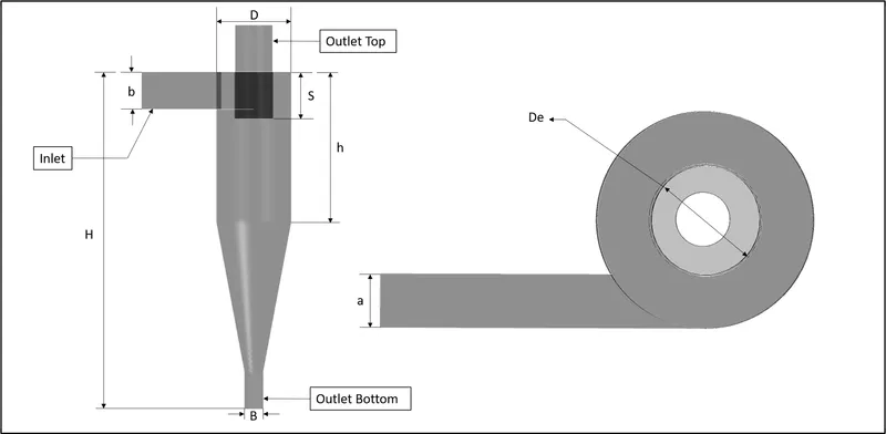
Fig. 1: Fluid Volume Model and Boundary Conditions regions wherein dimensions can be related to Section 1.1 Iozia and Leith Model (Image recreated with regards to reference research paper for correlational purposes only and does not intend to infringe on the copyrights of the original authors and their publication. Courtesy: A CFD Study on the Prediction of Cyclone Collection Efficiency)
2.2 Meshing
The meshing approach adopted for the given computational domain was developed to maintain the meshing quality attributes viz., element quality, skewness, orthogonality, and aspect ratio within the ranges as laid out in the Meshing training material of ANSYS outlined in the following table:
|
Element Quality |
0 (Bad Mesh) |
1 (Good Mesh) |
||||
|
Aspect Ratio |
Triangles |
1 (for an equilateral triangle) |
- Best possible value |
|||
|
Quadrilaterals |
1 (for a square) |
- Best possible value |
||||
|
Skewness |
0-0.25 (Excellent) |
0.25-0.50 (Very Good) |
0.50-0.80 (Good) |
0.80-0.94 (Acceptable) |
0.95-0.97 (Bad) |
0.98-1.00 (Unacceptable) |
|
Orthogonal Quality |
0-0.001 (Unacceptable) |
0.001-0.14 (Bad) |
0.15-0.20 (Acceptable) |
0.20-0.69 (Good) |
0.70-0.95 (Very Good) |
0.95-1.00 (Excellent) |
Table 1: Mesh Quality Attributes as defined in the ANSYS meshing training material
The reason for targeting the above mentioned mesh quality attributes comes from analysis across different types of geometries/models that these are few of the known ways of identifying whether the discretized mesh would face convergence issues during the solution process and also to locate areas in the mesh where the statistics can be improved. For each of the mesh, named selections such as inlet and outlet were created so as to assign their respective boundary conditions in the setup stage. Also, depending on the name of the named selection, Fluent is able to assign an inlet or outlet boundary condition with velocity-inlet and pressure-outlet type boundary conditions respectively which is a useful feature to have in flow-type problems of similar nature since the user now can only add values relating to the specific boundary condition thereby making the setup process a lot faster. In Sections 2.6.2 and 2.6.3, preparation about the different meshes have been discussed in detail along with their mesh qualities and the arrival on mesh independent solution.
2.3 CFD Simulation Setup, Boundary Conditions, Monitoring Points and Solution
The simulations on all meshes was performed using the Reynolds Averaged Navier-Stokes (RANS) models, in this case, the k-`epsilon` turbulence models and the discrete phase models. The use of k-`epsilon` turbulence models and more specifically the renormalization group (RNG) k-`epsilon` turbulence model is attributed to the fact that the Reynolds number, based on the given flow conditions, lies in the turbulence flow region, explained in Section 2.6.1 Evaluation of Reynolds number. For the given numerical analysis, the particle-laden flow wherein the particulate matter represents the dispersed phase while air as the continuous fluid phase within the cyclone separator is modelled as a gas-solid multiphase flow regime using the Lagrangian discrete phase model or quite simply, the discrete phase model. Additionally, all simulations were run using the double-precision feature as a general measure to resolve large variations in pressure differences. A brief description into the working of the k-`epsilon` turbulence model and discrete phase model is provided below:
2.3.1 k-`epsilon` turbulence model
The k-`epsilon` turbulence model is one of the first RANS turbulence models proposed by Launder and Spalding and is still being widely used for its robust, economic approach and reasonable accuracy in simulation of mean flow characteristics of large number of industrial flows and heat transfer applications. The k-`epsilon` turbulence model consists of two transport equations, one for the turbulent kinetic energy (k) to evaluate the energy in turbulence and the other is for the turbulent dissipation (`epsilon`) to calculate the rate of dissipation of turbulent kinetic energy (k). In this particular simulation, we will be performing simulations using the RNG k-`epsilon` model. The difference between the RNG k-`epsilon` and standard k-`epsilon` model can be described in the following two ways:
- Additional term in `epsilon` equation to improve accuracy for rapidly strained flows.
- Inclusion of effects of swirl on turbulence for swirling flows.
- Formulation of turbulent Prandtl numbers is analytical in comparison to the user-specified and constant values of standard k-`epsilon` model.
- Low-Reynold number effects are accounted because of the analytically derived differential formula for effective viscosity which is absent in the standard k-`epsilon` model definition making it effective mainly for high-Reynold number effects.
The above model based comparisons make the RNG k-`epsilon` turbulence model more appropriate for selection over a wider range of flows to the standard k-`epsilon` turbulence model and subsequently more accurate and reliable.
2.3.1.1 Setup of the RNG k-`epsilon` turbulence model:
To use the RNG k-`epsilon` turbulence model in the Fluent component system, we navigate to Viscous option in Models under the Physics Tab. In the Viscous Model feature, we choose k-`epsilon` (2 eqn) Model with type set to 'RNG', 'RNG Options' selected as 'Swirl Dominated Flow', based on the flow characteristics, and Near Wall treatment as 'Standard Wall Functions' which is the default option.
2.3.2 Discrete Phase Model
The discrete phase model, as mentioned before, conditions air as the continuous fluid phase by employing Navier-Stokes equations on it while the particulate matter as the dispersed phase is evaluated by tracking them through the developed flow field and this methodology is termed as the Euler-Lagrangian approach.
2.3.2.1 Setup of the Discrete Phase Model
Discrete phase model can be found in the Models section under the Physics Tab. In the discrete phase model window, 'Interaction with Continuous Phase' and 'Update DPM Sources Every Flow Iteration' options were checked with 'DPM Iteration Interval', and 'Max. Number of Steps' and 'Step Length Factor' in the 'Tracking Parameters' under the 'Tracking' tab retaining its default values of 10, 50000 and 5 respectively. 'Interaction with Continuous Phase' option allows for coupled calculations of the discrete phase with the continuous phase as interaction between them in the form of exchange of momentum exists. 'Update DPM Sources Every Flow Iteration' option performs calculation for source terms of particles at every iteration so as to ensure they reach their final values. 'DPM Iteration Interval' monitors the rate of tracking of the particles and updation of DPM sources which in the case of steady-state simulations increases stability with increasing number of intervals, however, number of iterations also increase towards attaining convergence. 'Max. Number of Steps' and 'Step Length Factor' evaluates trajectory of a single particle and monitors size of time step as part of the integration of equations of motion of a given particle respectively. The limit to the 'Max. Number of Steps' as 50,000, which also reflects the default value for the steady-state particle tracking, implies that the calculation of trajectory for any given particle injection beyond this value will be terminated and reported as "incomplete" thereby eliminating particles trapped in a recirculating region of the continuous phase field and avoiding their tracking indefinitely. The 'Step Length Factor' determines the time step value dependent on the time required by a dispersed phase particle to traverse the given continuous phase control volume. The discrete phase particle attributes were defined by clicking on the 'Injections' button and creating a new 'Injection' wherein the 'Injection Type' was set to 'surface', 'Release from Surfaces' was selected as 'Inlet', 'Particle Type' was chosen to be 'Inert' while 'Material' and 'Diameter Distribution' was retained to its default settings of 'anthracite' and 'uniform' respectively. As no specific domain was assigned for the discrete phase, the 'Discrete Phase Domain' option only contained the 'none' item. 'Injection Type' of 'surface' allows particles, typically possessing similar properties, to be allowed entry access of movement from a particular zone or region, in this case the 'Inlet', with the particles demonstrating inert nature that follows the force balance equations and behaves according to the Inert Heating or Cooling Laws. Input properties of the particles are defined explicitly under the 'Point Properties' section tab with values for velocity and diameter variables dependent on the governing conditions as described in the computational problem while total flow rate retaining its default value of 1e-20 kg/s. The other aspects of the discrete phase particle features include the 'Physical Models' with 'Drag Law' maintained at spherical indicating that the discrete phase is treated as smooth spherical particles while 'Stochastic Tracking' and 'Cloud Tracking' under 'Turbulent Dispersion' are not enabled even though the flow is turbulent as the effects of turbulence on particle dispersion was not being captured. Also, as there is no ascribed motion with regards to the given domain, there are no initialization parameters for the 'UDF' section tab.
2.3.3 Boundary Conditions and Monitoring Points
The different boundary conditions for the simulation of air and particulate matter within the cyclone separator model is described in the following table:
|
Named Selections |
inlet |
outlet_top |
outlet_bottom |
wall |
|
Type |
Velocity-inlet |
pressure-outlet |
pressure-outlet |
wall |
|
Velocity Specification Method |
Magnitude, Normal to Boundary |
-- |
-- |
-- |
|
Velocity Magnitude (m/s) |
1, 3 and 5 |
-- |
-- |
-- |
|
Turbulence Specification Method |
Intensity and Viscosity Ratio |
Intensity and Viscosity Ratio |
Intensity and Viscosity Ratio |
-- |
|
Turbulent Intensity (%) |
5 |
-- |
-- |
-- |
|
Turbulent Viscosity Ratio |
10 |
-- |
-- |
-- |
|
Pressure Profile Multiplier |
-- |
1 |
1 |
-- |
|
Backflow Direction Specification Method |
-- |
Normal to Boundary |
Normal to Boundary |
-- |
|
Gauge Pressure (Pa) |
-- |
0 |
0 |
-- |
|
Backflow Pressure Specification |
-- |
Total Pressure |
Total Pressure |
-- |
|
Backflow Turbulent Intensity (%) |
-- |
5 |
5 |
-- |
|
Backflow Turbulent Viscosity Ratio |
-- |
10 |
10 |
-- |
|
Wall Motion |
-- |
-- |
-- |
stationary wall |
|
Shear Condition |
-- |
-- |
-- |
no slip |
|
Discrete Phase BC type |
reflect |
escape |
trap |
reflect |
Table 2: Boundary Conditions including different velocity values representing different inlet flow conditions for simulation of particulate matter within the cyclone separator
Reflect discrete phase boundary condition type rebounds the discrete phase particles off a particular zone or region, in this case at the inlet and walls of the fluid volume domain, by affecting its inbound momentum and as the particles are non-rotating, the momentum is calculated with regards to the coefficient of restitution which states that the amount of momentum in normal direction to the wall is retained by the particle after collision with the boundary [7]. Escape type discrete phase boundary condition essentially leaves or exits out at the designated area, in this case at the top outlet region, and trajectory calculations for escaped particles are discontinued. The trap discrete phase boundary condition type enables the particles to be captured at a given zone, in this case at the bottom outlet region, and similar to the escape type discrete phase boundary condition, trajectory calculations are terminated.
For the given problem, the material properties for the continuous phase is retained as air by default with density value of 1.225 `(kg)/m^3`and the viscosity (or dynamic viscosity) value of `1.7894*10^(−5) (kg)/(ms)` while the discrete phase particle of material type inert uses anthracite having density value of 1550 `(kg)/m^3`. The material as air flowing through the fluid control volume can be verified by heading over to the "volume_volume" zone of "Cell Zones" under the "Zones" section of the "Physics" tab and click on "Edit" button for viewing the different attributes of the same. It should be noted that both the flow velocity and the particle velocity when defined in the boundary conditions and the 'Point Properties' section tab of the created 'Injection' respectively represent the same numerical values.
The choice of Turbulence specification method chosen for this simulation is Intensity and Viscosity Ratio wherein the Intensity (or Turbulent Intensity) is defined as the ratio of root-mean-square (RMS) value of velocity fluctuations to average flow velocity while Viscosity Ratio (or Turbulent Viscosity Ratio) is defined as the ratio of the turbulent viscosity to the laminar viscosity. Turbulent intensity is set to a value of 5% (representing medium intensity) and the Turbulent Viscosity Ratio has its default value at 10 since this value was not directly available from any experimental findings and in that case these values usually lie in a typically good scale or range as is recommended in the lecture series by ANSYS on Turbulence Modeling.
During the solution process, the area-weighted and volume average static pressure plots were monitored across the entire cyclone separator to observe stability in their respective values. The required monitoring plots were created from the 'Definitions' drop-down menu in the 'Reports' section of the 'Solution' tab and choosing 'Area-Weighted Average' option in the 'Surface Report' and 'Volume Average' option in the 'Volume Report' for static pressure by selecting 'Pressure' in the 'Field Variable' and 'Static Pressure' as the attribute, selecting all surfaces in the 'Wall Zones' list for the former and 'volume_volume' in the 'Cell Zones' list, checking the 'Report File' and 'Report Plot' boxes before clicking on the 'OK' button. Fig. 1 outlines the named selections where the boundary conditions would be employed as well as contour plots to demonstrate the axial, radial and tangential velocity and static pressure distributions discussed in Section 2.3.4 Solution.
2.3.4 Solution
The nature of given CFD simulation is steady while type of solver chosen is Pressure-based solver as we are dealing with a low-speed incompressible flow problem i.e., speed of fluid flow is typically in the subsonic range and density of material does not change or the change is almost negligible within the given control volume, although the Fluent Theory Guide also claims that the Pressure-based solver can now solve and operate beyond its previous limitations. The Pressure-based solver calculates the Pressure field by evaluating the pressure or pressure-correction equation that is determined from the manipulation of continuity and momentum equations. Velocity formulation is chosen to be absolute as the velocity in the given fluid control volume is not rotating. Since, the separation of particulate matter from air is influenced by the gravitational field, 'Gravity' option was enabled with y-axis as the reference direction and value in Y set to -9.81 `m/s^2` representing downward direction of gravitational acceleration on the system. To run the solution, the given fluid volume needs to be initialised which in this case is done using the 'Standard Initialisation' option. Standard Initialisation, as described in the Fluent Theory Guide, allows the user to specify all the variables directly as initial guess values across each cell of the entire domain. The variables can include initial guess values for velocity, temperature, pressure, etc. from the available list. In this case, the flow field is initialised by utilising the values set at the 'Inlet' in the 'Compute from' drop-down list with values corresponding to the same zone now available under the 'Initial Values' section. A contour plot to illustrate the static pressure, and axial, radial and tangential velocity gradients during the simulation run was setup and further used to record as their subsequent MPEG animation files. The contour plots were now available to be created under the 'Graphics' section of the 'Results' tab since the solution was initialized. After a new contour plot option was selected from the 'Contours' drop-down menu, a name was assigned, in this case, 'static-pressure' for 'Pressure' as the field variable with 'Static Pressure' as the attribute and similarly, 'axial-velocity', 'radial-velocity' and 'tangential-velocity' for 'Velocity' as the field variable with 'Velocity Magnitude' as the attribute, followed by clicking on the 'Filled' check-box and selecting all the surfaces in the 'Surfaces' list before clicking on the 'Save/Display' button. An animation plot of the same contours was created by heading back to the 'Solution' tab and clicking on the 'Solution Animations' option available under the 'Create' drop-down menu of the 'Activities' section. In the 'Animation Definition' window, the name of the animation was assigned as 'static-pressure-animation', 'axial-velocity-animation', 'radial-velocity-animation' and 'tangential-velocity-animation' with 'static-pressure', 'axial-velocity', 'radial-velocity' and 'tangential-velocity' chosen as the names of the contour plots respectively, on an individual basis, before clicking on 'OK'. Additionally, during the entire run, the default convergence criteria values were unaltered and disabled by selecting the 'Residuals' option in the 'Reports' section of the 'Solution' tab and unchecking the 'continuity', 'x-velocity', 'y-velocity', 'z-velocity', 'k', and '`epsilon`' for k-`epsilon` turbulence model to monitor the solution based on the number of iterations. Post-completion of the solution, a Particle Track (PT) file was created to visualise the trajectories of the particles in the dispersed phase using the post-processing software, CFD-Post, by accessing the 'Particle History Data' available in the 'Export' option of the 'File' menu item, selecting the 'Injection' item used during the simulation while ensuring the 'Quantity' and attribute are set to 'Particle Variables' and 'Particle Residence Time' respectively and assigning a 'Particle File Name' in the relevant directory before clicking on the 'Write' button.
2.4 Post-Processing
Visualisation of the particle trajectories was done by importing the PT file of the appropriate case using the 'Import' option of the 'File' menu item in CFD-Post with required transparency resolution set for the fluid volume to enable better representation of the dispersed phase. Additionally, 'Reduction Type' was set to 'Maximum Number of Tracks' with 'Max Tracks' changed to a value of 30 for clarity of envisioning of particle tracks. Legends have been added for 'Anthracite.Particle Time' plots with range opted as 'Local' to reflect the actual values of time corresponding to the last iteration within the domain for a better understanding of the graphical representation and can be viewed under Section 3 Results.
Expressions:
Area average pressure across the inlet (named selection) region:
Pressure Inlet = areaAve(Pressure)@inlet
Area average pressure across the outlet_bottom (named selection) region:
Pressure Outlet Bottom = areaAve(Pressure)@outlet_bottom
Area average pressure drop across the inlet and outlet_bottom (named selections) regions:
Pressure Drop = Pressure Inlet - Pressure Outlet Bottom
2.5 Reynolds number estimation, and Meshing strategy and Verification
In this numerical simulation, we have carried out verification of calculation (or mesh independence study) based on a minimum criteria of particles tracked as 250 during the solution process allowing for a more reliable cyclone separator efficiency calculation as well as comparing the minimum percentage variation (%var) in the predicted values of both the static pressure (Area-Weighted and Volumetric Average) quantities, more of which has been highlighted in Section 2.5.3 Mesh Refinement approach.
2.5.1 Evaluation of Reynolds number
There are two formulations of Reynolds number, one for the continuous fluid phase with regards to the cyclone separator and the other being the dispersed phase particle Reynolds number, also called as the relative Reynolds number. Turbulence characteristics for the governing flow conditions are determined based on the cyclone separator Reynolds number, the first formulation in the previous statement, and can be expressed as:
`Re = (rho*U_0*D)/mu`; where (Eq. 1)
`mu` is the dynamic viscosity of the fluid (in `(kg)/(m*s)`),
`rho` represents fluid density (in `(kg)/(m^3)`),
`D` is the cyclone diameter (in m), and
`U_0` is inlet flow velocity (in m/s)
The relative Reynolds number, based on the Fluent Theory Guide [7] documentation, can be expressed mathematically as:
`Re_r = (rho*d_p*|vec u_p- vec u|)/mu`; where (Eq. 2)
`mu` is the dynamic viscosity of the fluid (in `(kg)/(m*s)`),
`rho` represents fluid density (in `(kg)/(m^3)`),
`d_p` is the particle diameter (in m),
`vec u_p` is particle velocity (in m/s), and
`vec u` is fluid phase velocity
Substituting the inlet flow velocity, cyclone diameter, and density and dynamic viscosity of the fluid with values of 1m/s, 3m/s and 5m/s, 0.2m, and 1.225 `(kg)/m^3` and `1.7894*10^(−5) (kg)/(m*s)` respectively into (Eq. 1) to obtain the Cyclone Reynolds number, we get:
|
Inlet flow velocity (m/s) |
Cyclone Reynolds number (Re) (Eq. 1) |
|
1 |
13691.74 |
|
3 |
41075.22 |
|
5 |
68458.70 |
Table 3: Inlet flow velocity (m/s) and Cyclone Reynolds number (Re) for different flow configurations of the cyclone separator model
Since the values reported for the Cyclone Reynolds number in all three inlet flow velocity cases in Table 3 is greater than the limit defining turbulence of 4000 for internal flow simulation, it can be inferred that the flow lies in the turbulent regime.
2.5.2 Baseline Mesh
A baseline mesh, illustrated in Fig. 2, for the given computational domain was created with default element size of 0.055916m. For the given numerical analysis, three different schemes viz., SIMPLE, SIMPLEC and COUPLED, were compared to understand the effect on convergence and stability of the residuals and static pressure monitor plots as they are preferred algorithms for solving steady-state numerical problems unlike PISO which is generally used for transient calculations with large time steps. A detailed description of each of the three schemes have been mentioned in Section 2.6 Convergence Level.
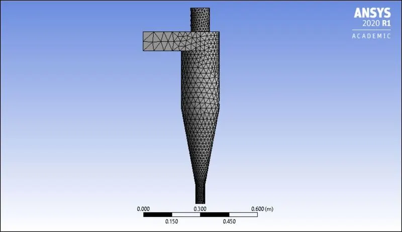
Fig. 2: Baseline Mesh
Mesh statistics and average static pressure values across the computational domain for Baseline Mesh using different Pressure-Velocity coupling schemes with flow and particle velocity values at 3m/s and particle diameter size of 5e-6m:
|
Mesh |
Mesh Element Size [m] |
Nodes |
Elements |
Pressure-Velocity Coupling Scheme |
Area-weighted average static pressure [Pa] |
Volumetric average static pressure [Pa] |
|
Baseline |
0.055916 |
4511 |
20362 |
SIMPLE |
5.484 |
4.320 |
|
Baseline |
0.055916 |
4511 |
20362 |
SIMPLEC |
5.472 |
4.315 |
|
Baseline |
0.055916 |
4511 |
20362 |
COUPLED |
5.467 |
4.313 |
Table 4: Mesh statistics and average static pressure values across the computational domain for Baseline Mesh using different Pressure-Velocity coupling schemes with flow and particle velocity values at 3m/s and particle diameter size of 5e-6m
Mesh quality attributes for Baseline Mesh:
|
Mesh |
Element Quality(avg.) |
Aspect Ratio(avg.) |
Skewness(avg.) |
Orthogonal Quality(avg.) |
|
Baseline |
0.82186 |
Triangles-1.9518 |
0.24699 |
0.75103 |
Table 5: Mesh quality attributes depicting average values of element quality, aspect ratio, skewness and orthogonal quality for Baseline mesh of the cyclone separator model
2.5.3 Mesh Refinement approach
The initial results obtained from the Baseline mesh in Section 2.5.2 Baseline Mesh with regards to the convergence behaviour of the three different algorithms, SIMPLE, SIMPLEC and COUPLED, as can be seen in Fig. 7, Fig. 8, and Fig. 9 respectively, it was observed that all monitor plots demonstrated highly stable outputs around the 100-300 iteration levels which is well before they reach the total number of initial iterations of 600, however, the COUPLED solver performed better than the two previously stated algorithms in terms of reporting the lowest value of residuals as opposed to the convergence limits mentioned in Table 8 (although the convergence criteria option for all equations were checked off) making the results obtained more reliable and accurate for it to be reused to solve the pressure-velocity equations for the four different meshes that were prepared to obtain a mesh independent solution. It is important to note that the maximum skewness reported for the Baseline Mesh by Fluent was 0.98288, which is more than the recommended value of 0.98 (highly skewed cells lead to convergence difficulties, decreased accuracy and unstable solution), and while results with SIMPLE and SIMPLEC schemes may have varied for a mesh with reduced skewness, the purpose of the Baseline Mesh was to guide towards an improved mesh refinement strategy that ensured not only the underlying physics was well captured but also the results were at least in close proximity to the default convergence criteria. The mesh refinement hereafter was created, while adhering to the mesh quality attributes mentioned in Section 2.2 Meshing, with only the mesh element size being reduced by 20%, in every subsequent mesh iteration, to minimize errors due to numerical diffusion that eventually led to uniform division of the meshing elements and consequently reduced skewness. Additionally, an attempt to create a structural mesh by using cutcell meshing approach to reduce number of meshing elements and simultaneously improve the meshing quality to yield better results in terms of number of particles tracked was tried. However, the assembly meshing method failed to work for an unknown and unaccountable reason with local body sizing method for smaller element sizes as the number of meshing elements remained unaffected and therefore, the unstructured meshing approach was continued towards achieving a mesh independent result as well as for simulation of different particle diameter sizes, and particle and flow velocity cases.
Mesh 1:
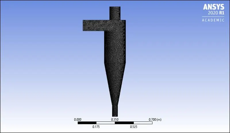
Fig. 3: Mesh 1
Mesh 2:
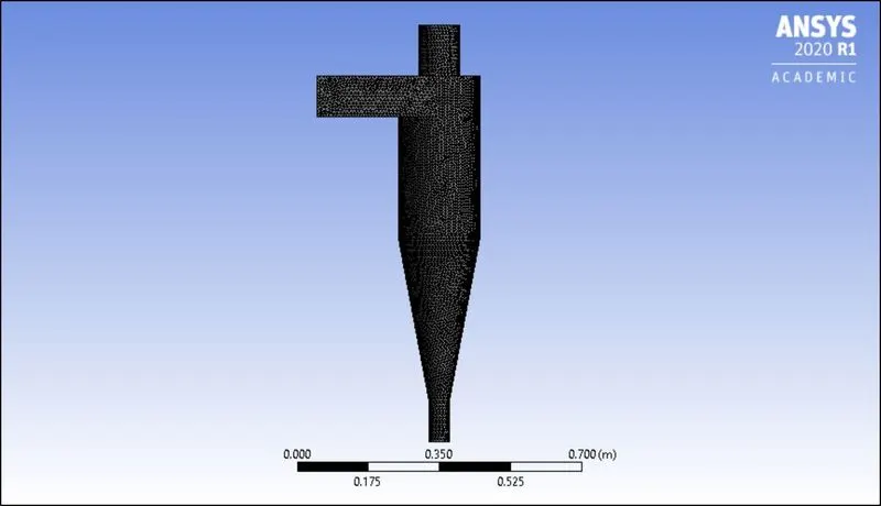
Fig. 4: Mesh 2
Mesh 3:
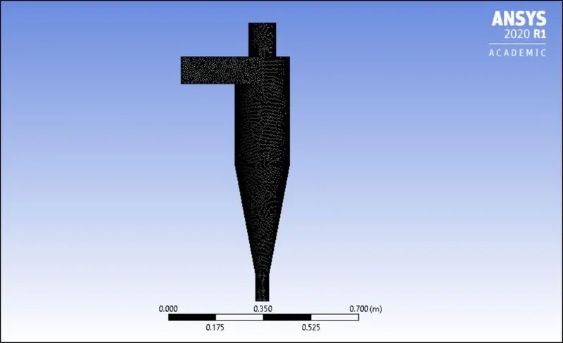
Fig. 5: Mesh 3
Mesh 4:
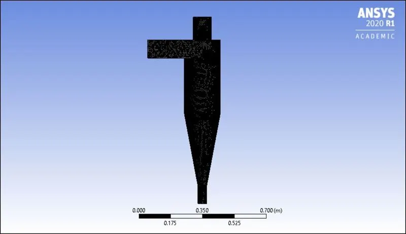
Fig. 6: Mesh 4
Mesh statistics and average static pressure values across the computational domain for different meshes using COUPLED Pressure-Velocity coupling scheme with flow and particle velocity values at 3m/s and particle diameter size of 5e-6m:
|
Mesh |
Mesh Element Size [m] |
Nodes |
Elements |
Area-weighted average static pressure [Pa] |
%var |
Volumetric average static pressure [Pa] |
%var |
No. of Particles tracked |
|
1 |
0.01 |
22951 |
112565 |
11.899 |
-- |
9.366 |
-- | 124 |
|
2 |
0.008 |
37119 |
185349 |
13.580 |
+14.127 |
10.631 |
+13.506 | 172 |
|
3 |
0.0064 |
62836 |
319221 |
15.404 |
+13.431 |
12.031 |
+13.169 | 276 |
|
4 |
0.0053 |
97701 |
502034 |
16.624 | +7.92 | 12.956 | +7.688 | 360 |
Table 6: Mesh statistics and average static pressure values across the computational domain for different meshes using COUPLED Pressure-Velocity coupling scheme with flow and particle velocity values at 3m/s and particle diameter size of 5e-6m
Mesh quality attributes for the four different meshes:
|
Mesh |
Element Quality(avg.) |
Aspect Ratio(avg.) |
Skewness(avg.) |
Orthogonal Quality(avg.) |
|
1 |
0.83691 |
Triangles - 1.8571 |
0.22862 |
0.76952 |
|
2 |
0.83779 |
Triangles - 1.8513 |
0.22746 |
0.77072 |
|
3 |
0.83845 |
Triangles - 1.8484 |
0.22629 |
0.77193 |
|
4 |
0.83893 |
Triangles - 1.845 |
0.22589 |
0.77236 |
Table 7: Mesh quality attributes depicting average values of element quality, aspect ratio, skewness and orthogonal quality for different meshes of the cyclone separator model
From the meshing statistics in Table 6, mesh number 3 (or mesh 3) with 319221 elements represents a mesh independent result in terms of minimum percentage variation (%var) in the predicted values of both the static pressure (Area-Weighted and Volumetric Average) quantities. The %var is calculated as the ratio of the difference of the predicted values in two consecutive meshes to the predicted value of the previous mesh e.g., ((Area-Weighted Average of static pressure for Mesh 2 - Area-Weighted Average of static pressure for Mesh 1)/Area-Weighted Average of static pressure for Mesh 1). Due to constraints in computational resources and limitations in maximum number of cells/nodes for solution by ANSYS Student license to 512,000 any further reduction in values of mesh element size was not possible to achieve for the given numerical analysis. Also, apart from mesh 1 with element size of 0.01m reporting a maximum skewness value of 0.98074, all other meshes with regards to realising a mesh independent result outlined maximum skewness value of less than 0.98. Results in Section 3 will only be referred with regards to the mesh independent solution i.e., Mesh 3.
2.6 Convergence Level
As mentioned earlier in Section 2.5.2 Baseline Mesh, three different schemes i.e., SIMPLE, SIMPLEC and COUPLED were compared with regards to convergence study. SIMPLE scheme is iterative in nature, robust (memory efficient) and is quicker per iteration than other pressure-based solvers. SIMPLEC scheme, similar to the SIMPLE scheme, allows increased under relaxation to the pressure correction term that improves in convergence times especially when employed in complicated flows with turbulence and/or supplementary physical models and as such offers greater diversity in terms of computational problems for implementation over SIMPLE scheme. While SIMPLE and SIMPLEC schemes are segregated type of schemes i.e., pressure and velocity terms are updated sequentially, the COUPLED scheme on the other hand updates the pressure and velocity terms simultaneously. This allows the COUPLED scheme to be more efficient in its single-phase implementation especially for steady-state flows offering superior performance over the segregated algorithms (SIMPLE and SIMPLEC) thereby requiring fewer iterations to converge. The selection of schemes for the different terms under spatial discretization includes assigning Gradient to Least Squares Cell Based scheme, pressure to second order scheme, and momentum, Turbulent Kinetic Energy and Turbulent Dissipation Rate to second order upwind scheme. Least Squares Cell Based scheme is the default gradient method chosen by ANSYS Fluent which is used to compute the change in values across the centroid of two cells along a vector path and is a computationally less expensive scheme offering comparable accuracy to the node-based gradient scheme, both of which are superior to the cell-based gradient scheme. The second order scheme for the pressure makes use of the central differencing scheme and is generally considered to be more accurate than the Standard and Linear schemes as well as robust in the case of skewed meshes. A second order upwind scheme is chosen for the momentum and turbulence terms viz., Turbulent Kinetic Energy and Turbulent Dissipation Rate, that makes use of the quantities at the cell face values to compute a cell-centered solution at the cell centroid leading to a second order accurate solution. Convergence criteria option was checked off, however, the residual values which measures the local imbalance of conserved variable in each control volume such as continuity, x-velocity, y-velocity, z-velocity, k, and `epsilon` were monitored throughout the solution process for the defined number of iterations i.e., 1000, to allow for the development of the flow behaviour which is the separation of the dispersed phase particles from the continuous fluid phase of air. The residual limits defined for the turbulence model equations, and the residual and monitor plots corresponding to the different meshes are shown in the table and figures below respectively:
|
k-`epsilon` |
|
|
continuity |
1e-03 |
|
x-velocity |
1e-03 |
|
y-velocity |
1e-03 |
|
z-velocity |
1e-03 |
|
k |
1e-03 |
|
`epsilon` |
1e-03 |
Table 8: Residual Values of the different equations used in the RNG k-`epsilon` turbulence model
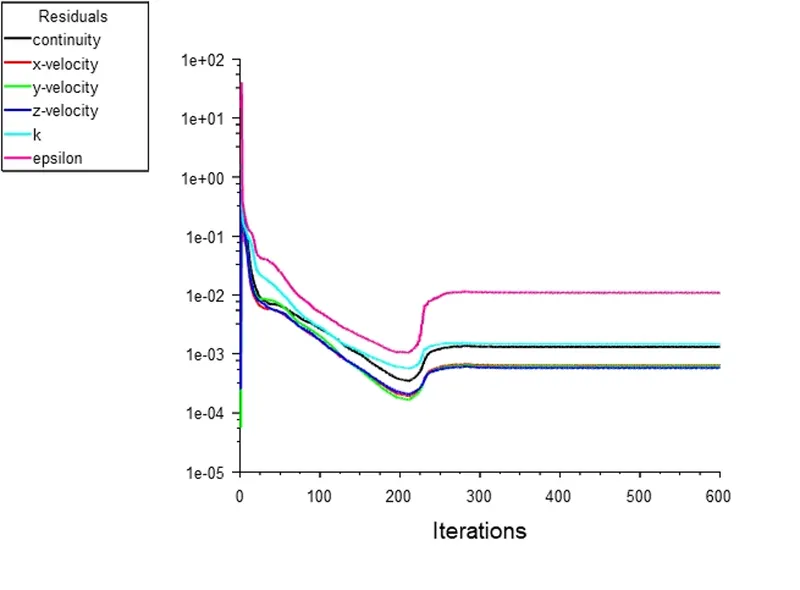
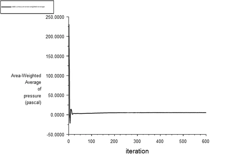
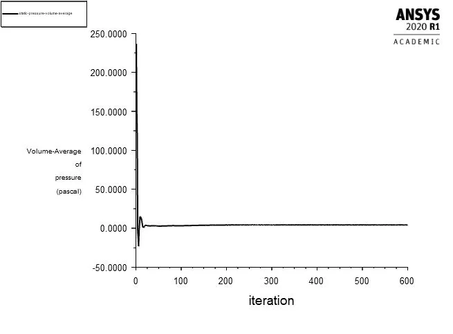
Fig. 7: Scaled Residuals and Static Pressure (Area-Weighted and Volumetric Average) plots for Baseline mesh using the RNG k-`epsilon` turbulence model with SIMPLE solver, particle and flow velocity at 3m/s and particle diameter size of 5e-6m
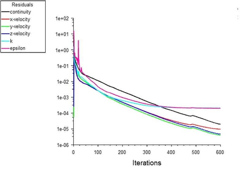
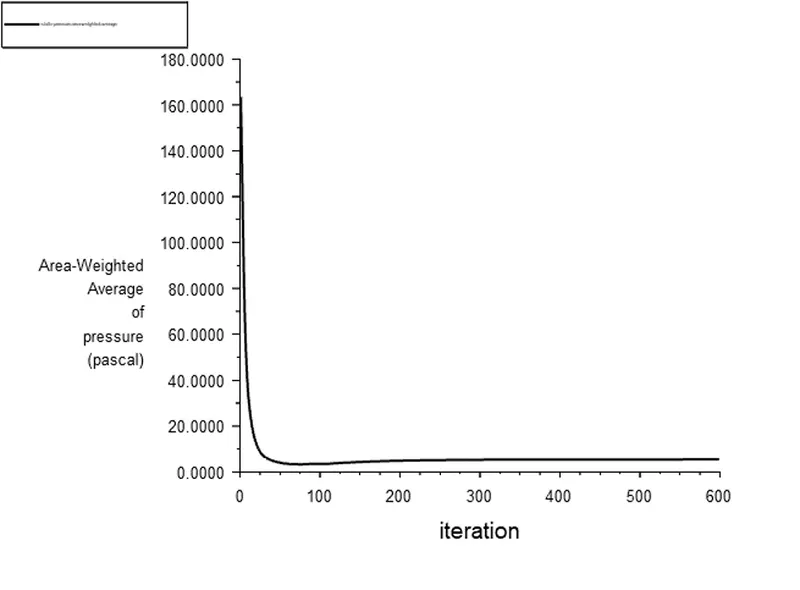
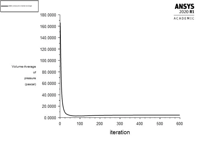
Fig. 8: Scaled Residuals and Static Pressure (Area-Weighted and Volumetric Average) plots for Baseline mesh using the RNG k-`epsilon` turbulence model with SIMPLEC solver, particle and flow velocity at 3m/s and particle diameter size of 5e-6m
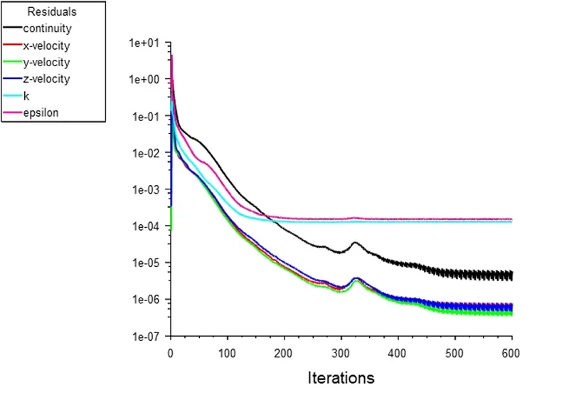
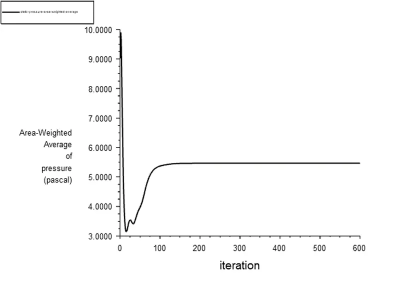
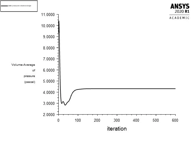
Fig. 9: Scaled Residuals and Static Pressure (Area-Weighted and Volumetric Average) plots for Baseline mesh using the RNG k-`epsilon` turbulence model with COUPLED solver, particle and flow velocity at 3m/s and particle diameter size of 5e-6m
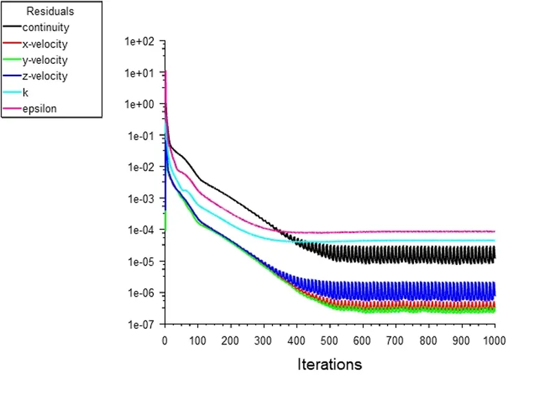
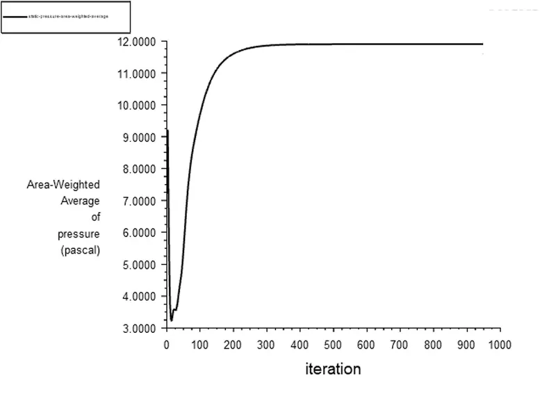
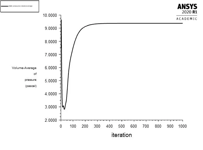
Fig. 10: Scaled Residuals and Static Pressure (Area-Weighted and Volumetric Average) plots for mesh 1 using the RNG k-`epsilon` turbulence model with COUPLED solver, particle and flow velocity at 3m/s and particle diameter size of 5e-6m
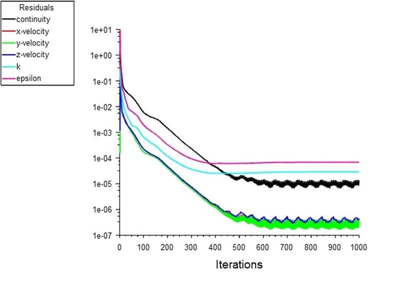
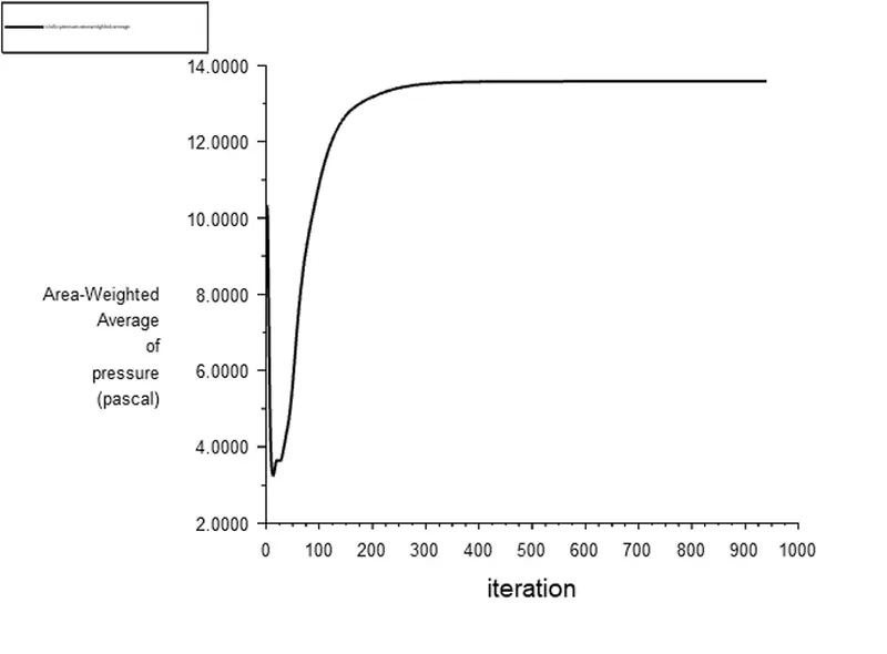
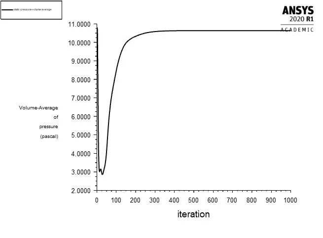
Fig. 11: Scaled Residuals and Static Pressure (Area-Weighted and Volumetric Average) plots for mesh 2 using the RNG k-`epsilon` turbulence model with COUPLED solver, particle and flow velocity at 3m/s and particle diameter size of 5e-6m
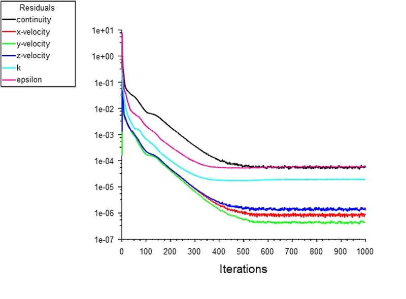
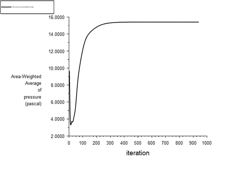
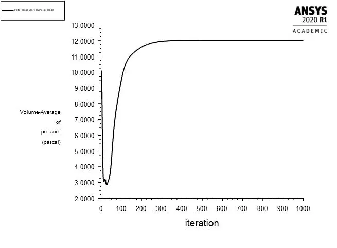
Fig. 12: Scaled Residuals and Static Pressure (Area-Weighted and Volumetric Average) plots for mesh 3 using the RNG k-`epsilon` turbulence model with COUPLED solver, particle and flow velocity at 3m/s and particle diameter size of 5e-6m
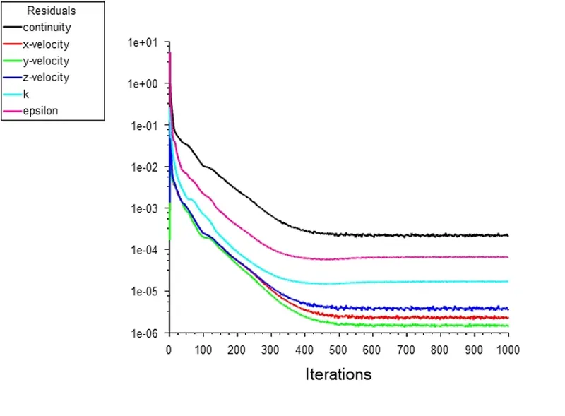
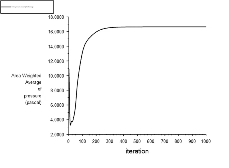
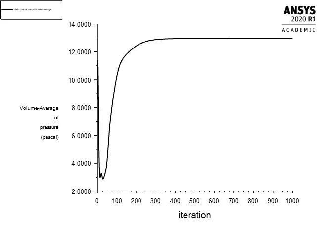
Fig. 13: Scaled Residuals and Static Pressure (Area-Weighted and Volumetric Average) plots for mesh 4 using the RNG k-`epsilon` turbulence model with COUPLED solver, particle and flow velocity at 3m/s and particle diameter size of 5e-6m
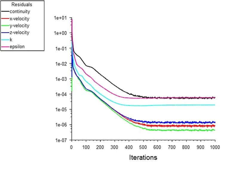
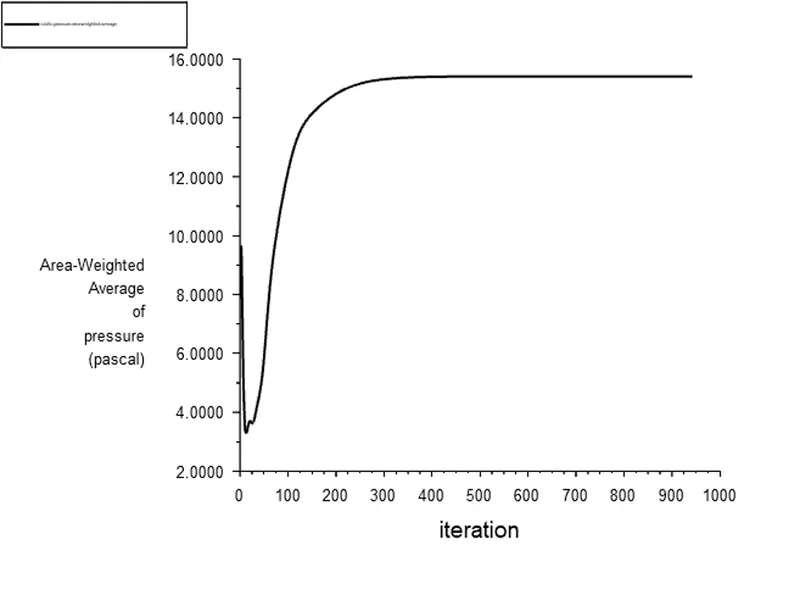
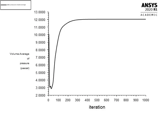
Fig. 14: Scaled Residuals and Static Pressure (Area-Weighted and Volumetric Average) plots for mesh 3 using the RNG k-`epsilon` turbulence model with COUPLED solver, particle and flow velocity at 3m/s and particle diameter size of 1e-6m
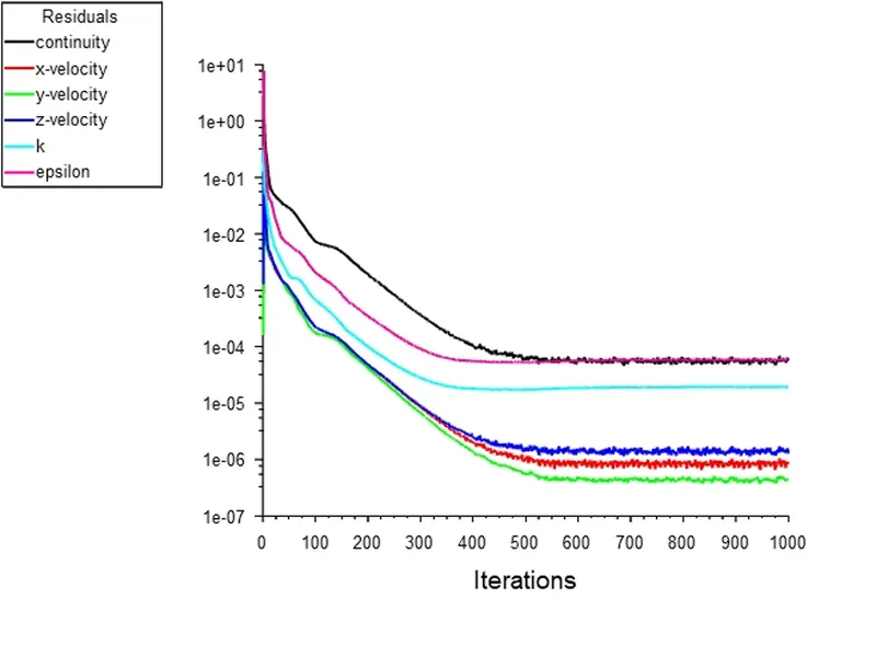
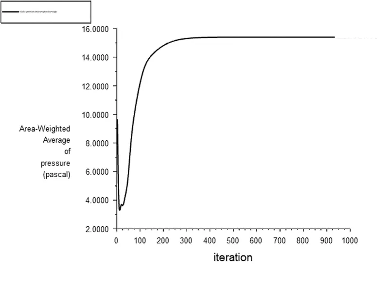
Fig. 15: Scaled Residuals and Static Pressure (Area-Weighted and Volumetric Average) plots for mesh 3 using the RNG k-`epsilon` turbulence model with COUPLED solver, particle and flow velocity at 3m/s and particle diameter size of 3e-6m
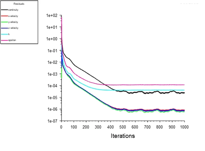
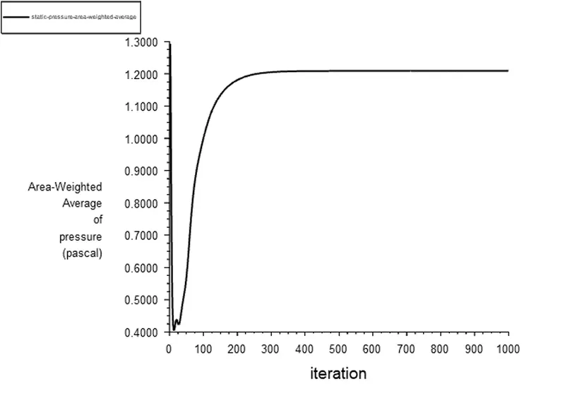
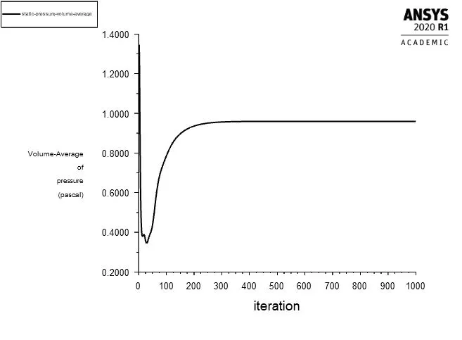
Fig. 16: Scaled Residuals and Static Pressure (Area-Weighted and Volumetric Average) plots for mesh 3 using the RNG k-`epsilon` turbulence model with COUPLED solver, particle and flow velocity at 1m/s and particle diameter size of 5e-6m
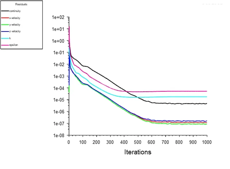
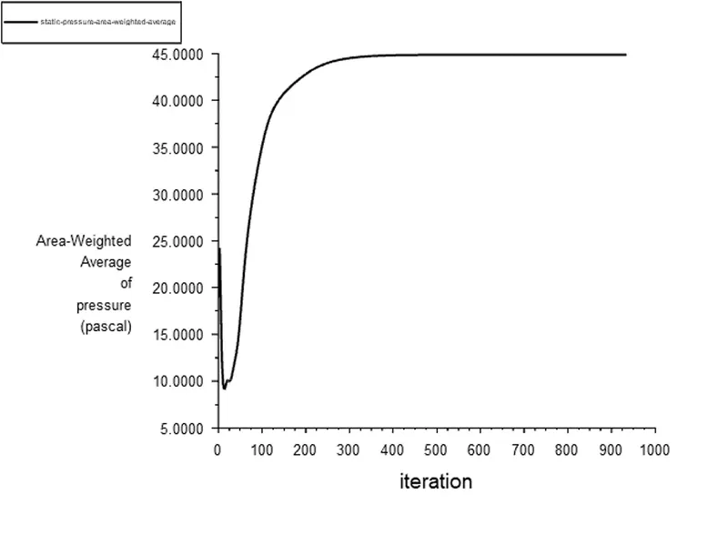
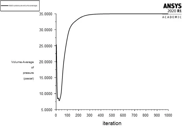
Fig. 17: Scaled Residuals and Static Pressure (Area-Weighted and Volumetric Average) plots for mesh 3 using the RNG k-`epsilon` turbulence model with COUPLED solver, particle and flow velocity at 5m/s and particle diameter size of 5e-6m
From Fig. 7, Fig. 8 and Fig. 9, it can be noticed that all three of the pressure-velocity coupling schemes have shown stable convergence with highly stable outputs as seen in the monitor plots well before they reach the total number of iterations indicating that a steady-state solution was obtained, however, the COUPLED scheme, as was also mentioned in Section 2.5.3 Mesh Refinement approach, has the lowest recorded residual limit values while also taking the most computational time. This reconfirms the expected behaviour from each of the schemes. A similar trend in results is also observed from Fig. 10 to Fig. 17 in the simulation of different meshes and case setup with regards to the particle diameter sizes, and particle and flow velocities, except a few residuals expressing small amplitudes of oscillatory fluctuations and the output of the monitor plots varying with respect to the numerical values.
3.Results
In Section 3.1, velocity (axial, radial and tangential) and static pressure contour animation plots, and anthracite particle time contour plots for different particle diameter sizes and particle and flow velocities are highlighted along with tabulated information for number of particles tracked, trapped, escaped and incomplete as well as calculations for cyclone separator efficiency and pressure drop.
3.1 Numerical results for cyclone separator efficiency and pressure drop for different particle diameter sizes and particle and flow velocities
Cyclone separator efficiency is evaluated as the percentage ratio of number of particles tracked to the number of particles trapped and is expressed as:
`eta = (NP_(trapped))/(NP_(tracked))*100` (Eq. 3)
Pressure drop in a cyclone separator can be realised as a function of the dimensions of the device and its operating conditions and its variation is dependent on changes to area, friction on the walls, direction of flow, dissipation in the outlet tube (also known as the vortex finder). This leads to classification of pressure drop as entry pressure loss in the tangential inlet duct, frictional loss for the travel along the spiral distance in the outer vortex, pressure loss due to change of air flow direction from outer to inner vortex, and entry pressure loss between air entering the inner vortex and leaving the outlet tube. For the given computational problem and for simplification reasons, the pressure drop was calculated as the difference in pressure values at the inlet and outlet bottom named selections, as also mentioned in Expressions under Section 2.4 Post-Processing, for each of the simulated cases.
3.1.1 Effect of different particle diameter sizes
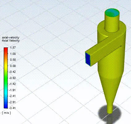
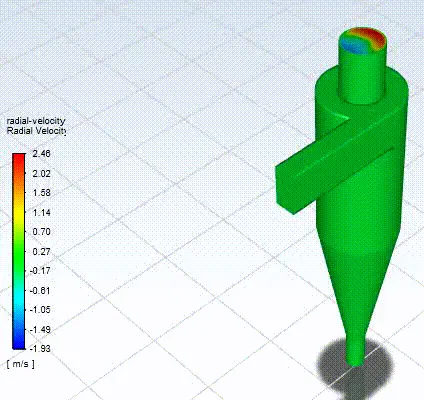
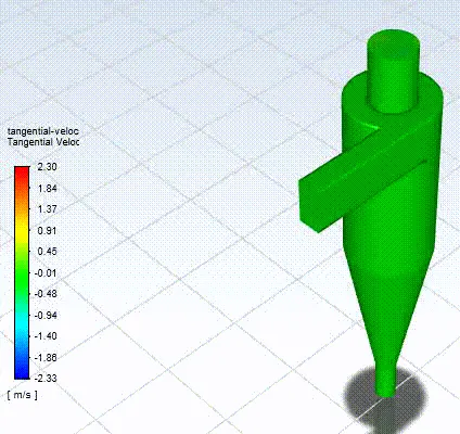
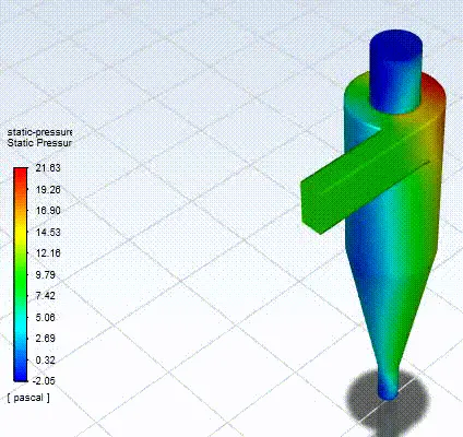
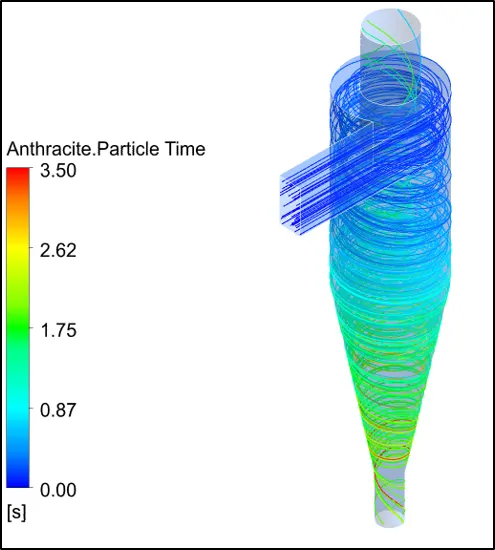
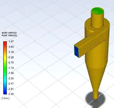
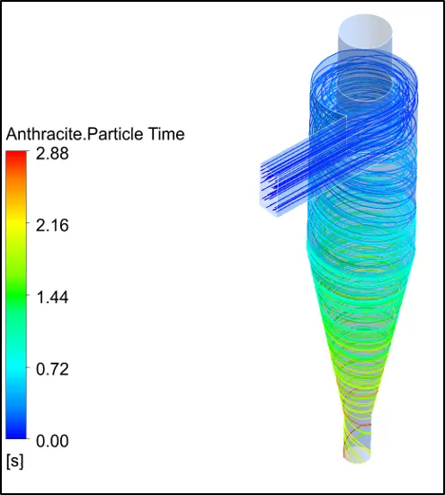
Fig. 18, Fig. 19, and Fig. 20 shows the velocity (axial, radial and tangential) and static pressure contour animation plots, and anthracite particle time contour plots for particle diameter sizes of 1, 3 and 5 micrometres at constant particle and flow velocity of 3m/s. Also, Table 9 indicates data on number of particles tracked, trapped, escaped and incomplete, as well as the corresponding cyclone separator efficiency and pressure drop relating to the same particle diameter sizes of 1, 3 and 5 micrometres, and particle and flow velocity of 3m/s. It can be seen that with increase in the particle diameter size from 1 to 5 micrometres, the anthracite particle time reduces as the particles have gained substantially more inertia allowing them to be less influenced by the presence of the swirling vortex. The increasing inertia attributed to the particle diameter size also displays the steadily growing impact on the cyclone separator efficiency as more particles get trapped thus indicating the preferred range in which the given cyclone separator model may work more appropriately. Since, the input velocity remains consistent in all three simulated cases, the three components of velocity i.e., axial, radial and tangential, and static pressure show similar contour plots implying that change in the particle diameter size may not have a strong presence on the pressure drop conditions.
For Mesh 3:
a) Axial velocity b) Radial velocity c) Tangential velocity
d) Static Pressure e) Anthracite Particle Time
Fig. 18: Velocity (axial, radial and tangential) and static pressure contour animation plots, and anthracite particle time contour plot for particle diameter size of 1 micrometre and particle and flow velocity of 3m/s
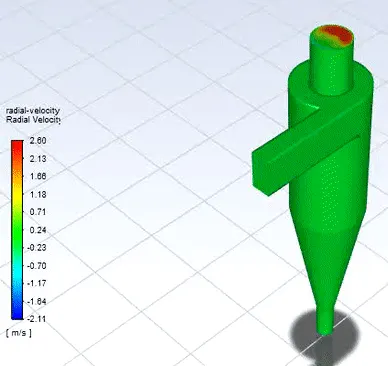
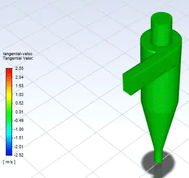
a) Axial velocity b) Radial velocity c) Tangential velocity
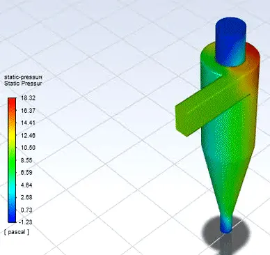
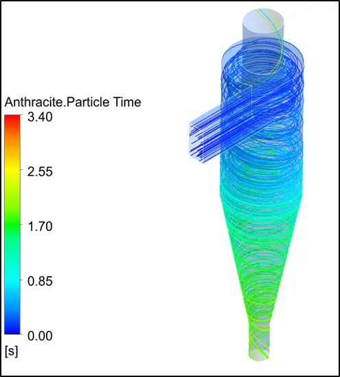
d) Static Pressure e) Anthracite Particle Time
Fig. 19: Velocity (axial, radial and tangential) and static pressure contour animation plots, and anthracite particle time contour plot for particle diameter size of 3 micrometre and particle and flow velocity of 3m/s
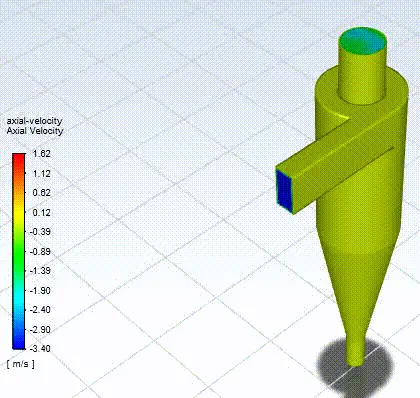
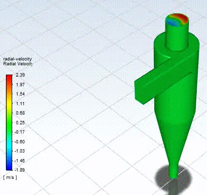
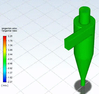
a) Axial velocity b) Radial velocity c) Tangential velocity
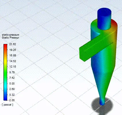
d) Static Pressure e) Anthracite Particle Time
Fig. 20: Velocity (axial, radial and tangential) and static pressure contour animation plots, and anthracite particle time contour plot for particle diameter size of 5 micrometre and particle and flow velocity of 3m/s
|
Input Velocity [m s^-1] |
Particle Diameter Size [m] |
Particles tracked |
Particles trapped |
Particles incomplete |
Particles escaped |
Cyclone separator efficiency (%) (Eq. 3) |
Pressure Drop [Pa] |
|
3 |
1e-6 |
276 |
67 |
155 | 54 |
24.275 |
23.1843 |
|
3 |
3e-6 |
276 |
235 |
15 |
26 |
85.145 |
23.1843 |
|
3 |
5e-6 |
276 |
257 |
19 | 0 |
93.116 |
23.1843 |
Table 9: Number of particles tracked, trapped, escaped and incomplete, and cyclone separator efficiency and pressure drop for the given cyclone separator model at different particle diameter sizes and same particle and flow input velocity of 3m/s
3.1.2 Effect of different particle and flow velocities
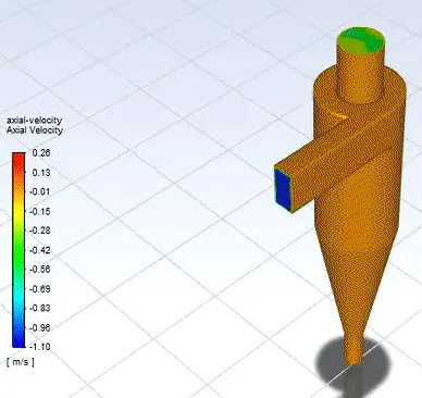
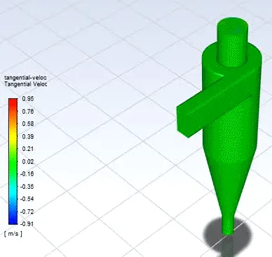
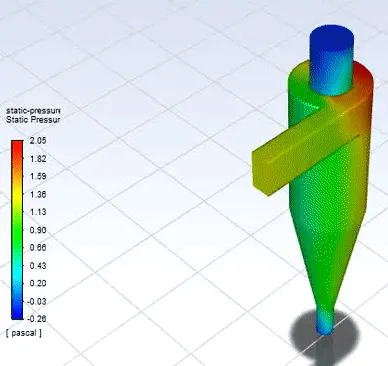
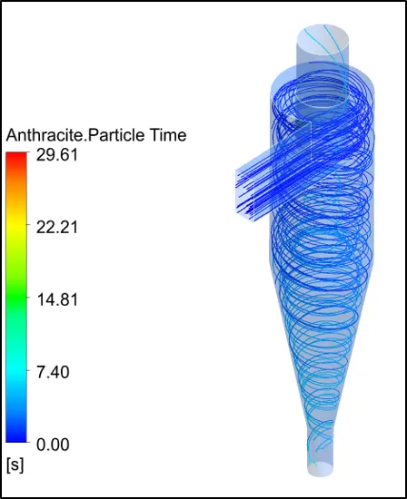
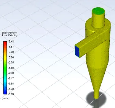
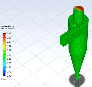
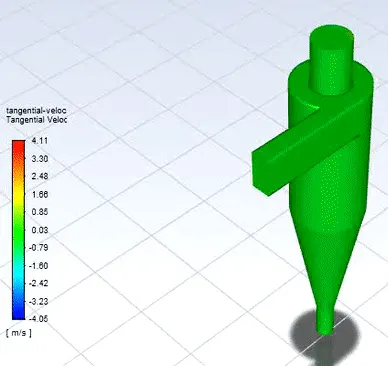
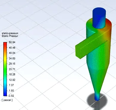
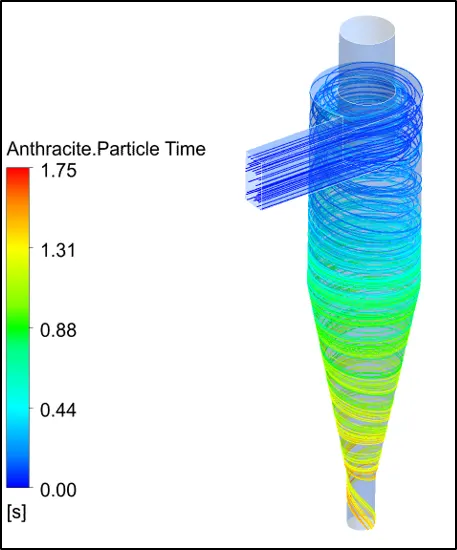
Fig. 21 and Fig. 22 shows the velocity (axial, radial and tangential) and static pressure contour animation plots, and anthracite particle time contour plots for particle diameter size of 5 micrometre at particle and flow velocities of 1m/s and 5m/s. Also, Table 10 indicates data on number of particles tracked, trapped, escaped and incomplete, as well as the corresponding cyclone separator efficiency and pressure drop relating to the same particle diameter size of 5 micrometre, and particle and flow velocities of 1m/s and 5m/s. The anthracite particle time is directly related to the change in velocity and decreases as the particles and flow velocities increases as time taken for the particles to traverse the device from the inlet and reach the outlet boundaries is reduced. A remarkable difference is noticed in the cyclone separator efficiency going from 1.449% to 93.116% when velocity changes from 1m/s to 3m/s respectively while the difference is less for velocity altered from 3m/s to 5m/s and this may be ascribed to the exchange of momentum between the flow and particles increasing at higher velocities as well as increasing the inertia of the dispersed phase particles leading to improved cyclone separator efficiency. Also, it can be observed that the pressure drop significantly rises with increase in input velocities of flow and particles and it is an indication of the increasing power requirements to enable consistent movement of the particle laden fluid through the cyclone separator.
a) Axial velocity b) Radial velocity c) Tangential velocity
d) Static Pressure e) Anthracite Particle Time
Fig. 21: Velocity (axial, radial and tangential) and static pressure contour animation plots, and anthracite particle time contour plot for particle diameter size of 5 micrometre and particle and flow velocity of 1m/s
a) Axial velocity b) Radial velocity c) Tangential velocity
d) Static Pressure e) Anthracite Particle Time
Fig. 22: Velocity (axial, radial and tangential) and static pressure contour animation plots, and anthracite particle time contour plot for particle diameter size of 5 micrometre and particle and flow velocity of 5m/s
|
Input Velocity [m s^-1] |
Particle Diameter Size [m] |
Particles tracked |
Particles trapped |
Particles incomplete |
Particles escaped |
Cyclone separator efficiency (%) (Eq. 3) |
Pressure Drop [Pa] |
|
1 |
5e-6 |
276 |
4 |
251 | 20 |
1.449 |
1.9557 |
|
3 |
5e-6 |
276 |
257 |
19 |
0 |
93.116 |
23.1843 |
|
5 |
5e-6 |
276 |
276 |
0 | 0 |
100 |
66.8549 |
Table 10: Number of particles tracked, trapped, escaped and incomplete, and cyclone separator efficiency and pressure drop for the given cyclone separator model at different particle and flow input velocities and same particle diameter sizes of 5e-6m
4. Discussion
Particle laden air enters the given reverse flow cyclone separator tangentially because of the positioning of the inlet and follows a spinning motion due to the geometrical features of the cylindrical upper body, conical bottom region and a smaller cylindrical section protruding from the top of the upper body to the outside, forming a double spiral wherein the outermost spiral follows a downward motion towards the exit of the dispersed phase particle while the innermost spiral moves upwards for the exit of the cleaner fluid. The dispersed phase particles being denser than the carrying fluid are driven towards the walls of the separator on account of the acting centrifugal forces while the less dense fluid (also particles depending on the diameter sizes and density) due to the impending drag forces from the flow remain entrained in the innermost vortex. Increasing velocities of flow and particles, especially the tangential component of velocity, increases the centrifugal forces causing more particles to collide against the walls of the separator, defined using the "no slip" condition, impeding the velocities of the particles to arrive at a value of 0m/s which are then drawn towards the bottom conical section under the influence of gravity. Tangential velocity behaves differently depending on the vortex in a manner that it increases with decrease of the rotational radius in the outer vortex while decreases with decrease in the rotational radius of the inner vortex such that the boundary between the two vortices can be deemed as its maximum value. Insufficiently low particle and flow velocities, even for large particle diameter sizes, creates an indefinite recirculation loop for the particles which leads them to remain within the device. Additionally, pressure field is generated by rotation of fluid flow within the separator with its highest value located at the walls and it decreases with reduction in rotational radius along the radial direction as tangential velocity increases causing a significant pressure drop and rise in radial acceleration.
5. Conclusion
The numerical analysis for cyclone separator model under steady state conditions for different input flow and particle velocities, and particle diameter sizes, using the RNG k-`epsilon` turbulence model and discrete phase model in ANSYS Fluent 2020 R1 was well understood. The creation of dispersed phase particles of different properties using particle injections as well as appropriate boundary conditions greatly assisted in recreating a commonly employed industrial level filtration or pre-filtration technique. Moreover, it was realised that the particle and flow properties, both particle diameter sizes and particle and flow velocities, impacted the efficiency and performance of the cyclone separator and investigations into the geometrical features of the device, as parameters for future research work, can greatly aid in optimising the design configuration aimed towards requirements of different applications.
5. References
[1] J. Gimbun, T. S. Y. Choong, A. Fakhru'l-Razi, A. L. Chuah, May 2005, "A CFD study on the Prediction of Cyclone Collection Efficiency", International Journal for Computational Methods in Engineering Science and Mechanics.
[2] Iozia, D. L., and Leith, D., Aerosol Sci. Technol. 12, 598 (1990).
[3] Barth, W., Brennstoff-Warme-Kraft, 8, 1 (1956).
[4] Li Enliang, and Wang Yingmin, A.I.Ch.E. J. 35, 666 (1989).
[5] Koch, W. H., and Licht, W., Chem. Eng., 7, 80 (1977).
[6] Lapple, C. E., Chem. Eng. 58, 144 (1951).
[7] ANSYS Fluent Theory Guide, Release 2020 R1 - © ANSYS, Inc. All rights reserved