Week 8: Literature review RANS derivation and analysis
Reynolds stress can be described as an additional component of stress developed as a consequence of the turbulent transport of momentum due to velocity fluctuations leading to subsequent deformation of fluid layers. The realisation of Reynolds stresses from a physical significance standpoint and its occurrence in the Reynolds-averaged Navier-Stokes equations for incompressible flow have been outlined in the following sections respectively.
Physical significance of Reynolds stresses:
The cause for Reynolds stresses from a physical perspective can be better understood by considering the following control volume consisting of a two-dimensional turbulent shear flow parallel to the x-axis along with a mean velocity gradient in the y-direction (Versteeg, H. K., & Malalasekera, W., 2007). A highly chaotic and intense mixing is generated due to the presence of swirling eddies that sets up random currents especially close to the bounding extents of the control volume leading to fluid transport across the same along with momentum and energy. Fig. 1 below exhibits the velocity gradient wherein the fluctuations containing negative y-velocity advance the fluid particles having higher x-momentum into the control volume across the top boundary as well as the fluid to a region of slower moving fluid across the bottom boundary while fluctuations with positive y-velocity, in general, would conversely create movement of slower moving fluid into higher velocity regions. In essence, the momentum exchange is a result of convective transport by eddies such that faster moving fluid layers would get decelerated while slower moving fluid layers accelerated leading to the influence of the additional turbulent shear stresses also known as the Reynolds stresses. Furthermore, temperature and concentration gradients would also lead to generation of turbulent heat or species concentration fluxes across the control volume domain bounding regions.
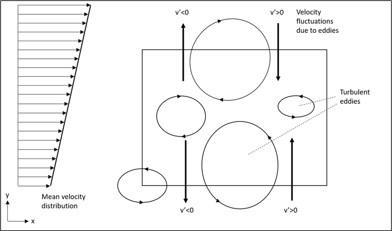
Fig. 1: Control volume within a two-dimensional turbulent shear flow (Adapted from [1])
Reynolds-averaged Navier-Stokes equations for incompressible flow (Versteeg, H. K., & Malalasekera, W., 2007):
The impact of turbulent fluctuations for mean flow equations for an incompressible flow with constant viscosity can be assessed by revisiting the assumptions for simplifying the algebra involved starting with the time averages of fluctuating properties followed by their summation, derivatives and integrals as shown below:
`varphi = Phi+ varphi'` `psi = Psi+ psi'`
`overline varphi' = overline psi' = 0` `overline Phi = Phi` `(overline (del varphi))/(del s) = (del Phi)/(del s)` `overline (int varphi ds) = int Phi ds` (Eq. 1)
`overline (varphi+psi) = Phi + Psi` `overline (varphi*psi) = Phi*Psi + overline (varphi'*psi')` `overline (varphi*Psi) = Phi*Psi` `overline (varphi'*Psi) = 0`
It is worth noting that the time-averaging option is nothing but integration and therefore, the order of time averaging and summation followed by further integration and/or differentiation can be swapped or commuted addressing this behaviour as a commutative property. As divergence and gradient are both differentiations, the rules mentioned above can be also utilised for a fluctuating vector quantity and its combinations with a fluctuating scalar as shown below:
`a = A + a'` `varphi = Phi+ varphi'`
`overline text(div)(a) = text(div) A`; `overline (text(div)(varphi*a)) = text(div)(overline (varphi*a)) = text(div)(Phi*A) + text(div)(overline (varphi'*a'))`; `overline (text(div) \ text(grad) \ varphi) = text(div) \ text(grad) \ Phi` (Eq. 2)
Let us consider the instantaneous continuity and Navier-Stokes equations with respect to Cartesian co-ordinate system such that the velocity vector `bb "u"` can be represented in three-dimensional space with x-component as `u`, y-component as `v` and z-component as `w` in the corresponding mathematical form as expressed below:
`text(div) \ bb "u" = 0` (Eq. 3)
`(del u)/(del t) + text(div) (ubb "u") = -1/rho*(del p)/(del x) + nu*text(div)(text(grad)(u))` (Eq. 4.a)
`(del v)/(del t) + text(div) (vbb "u") = -1/rho*(del p)/(del y) + nu*text(div)(text(grad)(v))` (Eq. 4.b)
`(del w)/(del t) + text(div) (wbb "u") = -1/rho*(del p)/(del z) + nu*text(div)(text(grad)(w))` (Eq. 4.c)
The above system of equations represents every turbulent flow characteristics, however, to understand the effects of turbulent fluctuations on the mean flow, Reynolds decomposition is used in the same set of equations i.e., (Eq. 3), (Eq. 4.a-c), along with replacing the flow and its space component variables viz., `bb "u"`, `u`, `v` and `w` and pressure `p` by the sum of a mean and fluctuating component as indicated mathematically below:
`bb "u" = bb "U" + bb "u"'` `u = U + u'` `v = V + v'` `w = W + w'` `p = P + p'` (Eq. 5)
Taking time average and applying the rules as observed in (Eq. 1) and (Eq. 2) to first the continuity equation in (Eq. 3), we get `text(div)\ bb "u" = text(div)\ bb "U"` and therefore the continuity equation for mean flow results into the following expression:
`text(div) \ bb "U" = 0` (Eq. 6)
Repeating the process for the x-momentum equation in (Eq. 4.a), the time averages of individual terms can be represented as shown below:
`overline (del u)/(del t) = (del U)/(del t)` `overline (text(div) (ubb "u")) = text(div)(Ubb "U") + text(div) overline ((u'bb "u'"))` `overline (-1/rho*(del p)/(del x)) = -1/rho*(del P)/(del x)` `overline (nu*text(div)(text(grad)(u))) = nu*text(div)(text(grad)(U))`
Simplifying (Eq. 4.a) by substituting the above set of time-averaged equations of individual terms in the x-momentum equation, a time-averaged x-momentum equation is arrived at as shown below:
`(del U)/(del t) + text(div)(Ubb "U") + text(div) overline ((u'bb "u'")) = -1/rho*(del P)/(del x) + nu*text(div)(text(grad)(U))` (Eq. 7.a)
Similarly, time-averaged y-momentum and z-momentum equations is obtained from (Eq. 4.b) and (Eq. 4.c) by repeating the process as adopted above for the x-momentum equation as shown below:
`(del V)/(del t) + text(div)(Vbb "U") + text(div) overline ((v'bb "u'")) = -1/rho*(del P)/(del y) + nu*text(div)(text(grad)(V))` (Eq. 7.b)
`(del W)/(del t) + text(div)(Wbb "U") + text(div) overline ((w'bb "u'")) = -1/rho*(del P)/(del z) + nu*text(div)(text(grad)(W))` (Eq. 7.c)
On a closer look at the first and second terms on both the left hand side and right hand side of (Eq. 7.a), (Eq. 7.b) and (Eq. 7.c), it can be noticed that the terms are similar to that appearing in (Eq. 4.a), (Eq. 4.b) and (Eq. 4.c), however, the time-averaging process has now added new terms representing the products of fluctuating velocities relating to the convective momentum transfer due to the presence of turbulent eddies viz., `text(div) (overline (text(space) \ text(component)'*bb "u'"))`. In order to indicate the presence of additional turbulent shear stresses on the mean flow, the terms indicating the products of fluctuating velocities is moved to the right hand side of their individual equations in (Eq. 7.a), (Eq. 7.b) and (Eq. 7.c) such that the simplified expressions can now be expressed as shown below:
`(del U)/(del t) + text(div)(Ubb "U") = -1/rho*(del P)/(del x) + nu*text(div)(text(grad)(U)) + 1/rho*[(del (-rho*overline (u'^2)))/(del x) + (del (-rho*overline (u'*v')))/(del y) + (del (-rho*overline (u'*w')))/(del z)]`(Eq. 8.a)
`(del V)/(del t) + text(div)(Vbb "U") = -1/rho*(del P)/(del y) + nu*text(div)(text(grad)(V)) + 1/rho*[(del (-rho*overline (u'*v')))/(del x) + (del (-rho*overline (v'^2)))/(del y) + (del (-rho*overline (v'*w')))/(del z)]` (Eq. 8.b)
`(del W)/(del t) + text(div)(Wbb "U") = -1/rho*(del P)/(del z) + nu*text(div)(text(grad)(W)) + 1/rho*[(del (-rho*overline (u'*w')))/(del x) + (del (-rho*overline (v'*w')))/(del y) + (del (-rho*overline (w'^2)))/(del z)]`(Eq. 8.c)
The additional turbulent stress components in (Eq. 8.a), (Eq. 8.b) and (Eq. 8.c) are represented in longhand form to represent the stress terms which are six in total with three normal stresses and three shear stresses as shown below:
Normal Stresses:
`tau_(text(xx)) = -rho*overline (u'^2)` `tau_(yy) = -rho*overline (v'^2)` `tau_(zz) = -rho*overline (w'^2)`
Shear Stresses:
`tau_(xy) = tau_(yx) = -rho*overline (u'*v')` `tau_(xz) = tau_(zx) = -rho*overline (u'*w')` `tau_(yz) = tau_(zy) = -rho*overline (v'*w')`
These extra turbulent stresses are known as the Reynolds stresses wherein the normal stresses consist of the respective variations in the velocity fluctuations along their spatial axes which would remain non-zero because of the squaring of the fluctuating terms while the shear stresses consist of second moments with regards to the correlations between different velocity components such that if two fluctuating velocity components like `u'` and `v'` were independent and random fluctuations, the resulting time average i.e., `overline (u'*v')`, would be zero, however, the structure of the vortical eddies does not lead to zero values of their turbulent stress components and are usually larger than the viscous stresses in turbulent flow. The equation set of (Eq. 6) and (Eq. 8.a - Eq. 8.c) is also known as the Reynolds-averaged Navier-Stokes equations (RANS).
Turbulent Viscosity:
To perform calculations for turbulent flows with RANS equations, it becomes imperative to create turbulence models that are able to predict the Reynolds stresses and scalar transport terms and thereby close the system of mean flow equations. In other words, the Reynolds stresses needs to be modelled as a function of the mean flow so as to avoid any reference to the fluctuating velocity components with such an approach giving rise to the commonly known closure problem. Boussinesq [2], a French mathematician and physicist, became the first individual to propose the eddy viscosity (or turbulent viscosity) concept in 1877 to deal with the closure problem wherein he suggested that the Reynolds stresses may be proportional to mean rates of deformation. This can be associated with experimental findings in which turbulence decays were observed unless shear is experienced in isothermal incompressible flows as well as increase in turbulence stresses as the mean rate of deformation increases. Eddy or turbulent viscosity defines the internal fluid friction created as a result of turbulent transfer of momentum by eddies prevalent within it while molecular viscosity, also referred to simply as viscosity, is the consequence of transport of mass motion momentum due to random and individual movement of molecules not combined in a group. An analogous relation can be considered between the molecular viscosity to the laminar flow and eddy or turbulent viscosity to the turbulent flow with the latter usually occurring on a much larger scale as seen in (Eq. 9) and (Eq. 10) below respectively, representing Newton's law of viscosity in the former wherein the viscous stresses is considered to be proportional to the rate of deformation of fluid elements and the same principles applied to the Reynolds stresses in the latter.
`tau_(ij) = mu_(ij) = mu*((del u_i)/(del x_j)+(del u_j)/(del x_i))`; where (Eq. 9)
`mu` is the molecular viscosity
`mu_(ij) = -rho*overline(u_i'*u_j') = mu_t*((del U_i)/(del x_j)+(del U_j)/(del x_i)) - 2/3*rho*k*delta_(ij)`; where (Eq. 10)
`mu_t` is the eddy or turbulent viscosity
References
[1] Versteeg, H. K., & Malalasekera, W. (2007). An introduction to computational fluid dynamics: The finite volume method (Eds.), Turbulence and its modelling (2nd ed., pp. 61–65). Harlow, England: Pearson Education Ltd.
[2] J. Boussinesq, Essai sur la théorie des eaux courantes, Mémoires présentés par divers savants à l’Académie des Sciences XXIII, 1 (1877) 1-680