Ahmed Body Challenge

1. Introduction

The recent advancements in the design of ground vehicles with regards to aesthetics, safety and most importantly the fuel economy has led to a rise in experimental and numerical studies to ascertain the contributing factors. In all such studies performed over the years, it was found that the aerodynamic drag of the vehicle impacted majorly on most design requirements and that the drag value was in turn governed by the wake region and the consequent structures developing within it beyond the rear end region of the vehicle as the air flow begins to separate from the vehicle surface.

The aim of this challenge is to perform steady-state simulations at an input velocity value of 25m/s to correlate the flow structures present in the wake for the given Ahmed Body model as a result of the flow separation and to calculate the coefficient of drag values. The Ahmed Body is a simplified car body proposed by S.R. Ahmed et. al [1] that consists of essentially three parts viz., a fore body, a mid-section and a rear end that looks similar to a rectangular cuboid containing rounded edges at the front and a slant face at the rear end. The reason behind this type of construction for the Ahmed Body was to reproduce essential physical features of a real world vehicle flow that can also be validated against experimental findings barring the exception of rotating wheels, engine and passenger compartment flow as well as the rough underside and vehicle surface projection regions. Also, the Ahmed Body model was ensured to have rounded fore body edges so as to achieve separated free flow over this surface which would result in most of the vehicle drag to be concentrated at the model's rear end. The analysis involves verification of the computed results with a mesh independence study detailing on the mesh refinement approach based on the 'y+' value, boundary layer thickness and required number of inflation layers to capture the boundary layer flow properties. The mesh independence study would also outline cell count, coefficient of drag values and number of iterations for convergence for each mesh based on stability of behaviour of coefficient of drag values as well as some of the mesh quality attributes like element quality, skewness, orthogonality, and aspect ratio. The mesh independent result would also be validated against the experimental value of coefficient of drag for the proposed Ahmed Body model configuration.

2. Method

2.1 Modelling

The computational domain for simulating flow around the given model for Ahmed Body was modelled in SpaceClaim, the default solid modeling CAD software for the Fluid Flow (Fluent) Analysis System. The extents of the computational model were estimated with respect to the LSTM low speed wind tunnel experiments performed by H. Lienhart et. al [2] and the recommendations in the ERCOFTAC workshop on Refined Turbulence Modelling [3] which included the length behind the Ahmed Body to be equivalent to five times the bluff body model length, length from the inlet to the bluff body as two times body length, overall width and height as five times the bluff body model width and height values respectively as illustrated in Fig. 1. This configuration of the computational model ensures a sufficient length for the incoming velocity profile to impose on the bluff body, negligible interaction of the outflow conditions with the bluff body wake and a blockage ratio of 4% (ratio of frontal projected area of the object viz., the bluff body, to the cross-sectional area of the domain surrounding the structure i.e., the wind tunnel, in the direction of flow) which is similar to the experimental setup [2]. Since, the computational domain has a uniform input flow of constant magnitude in all directions defined in a three-dimensional space, the simulations were carried out for one half of the model along the spanwise symmetry plane i.e., the model size was reduced for a faster computational time and more number of cells closer to the model walls. The extents for the computational model with regards to the bluff body dimensions were created using the "Enclosure" option under the "Prepare" tab in SpaceClaim. In order to perform calculations on one-half of the given setup along the spanwise symmetry plane, we create "Plane" available in "Create" section of the "Design" tab and select the origin of the model which is on the bluff body towards the front end. Then we use the "Split Body" command in the "Intersect" section under the "Design" tab and select the plane in the spanwise direction to split the bluff body and obtain the required symmetry model. This operation of creating a computational domain surrounding the Ahmed Body model and splitting the same along the spanwise symmetry plane is repeated to create a second enclosure closer to the bluff body with regards to mesh refinement which has been discussed in further details in Section 2.5 Verification.

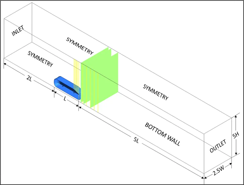
Fig. 1: Fluid Volume Model and Boundary Conditions regions (L, H and W refers to model length, height and width values respectively)

2.2 Meshing

The meshing approach adopted for the given computational domain was developed to maintain the meshing quality attributes viz., element quality, skewness, orthogonality, and aspect ratio within the ranges as laid out in the Meshing training material of ANSYS outlined in the following table:

Element Quality			0 (Bad Mesh)	1 (Good Mesh)
Aspect Ratio		Triangles	1 (for an equilateral triangle)	- Best possible value
		Quadrilaterals	1 (for a square)	- Best possible value
Skewness	0-0.25 (Excellent)	0.25-0.50 (Very Good)	0.50-0.80 (Good)	0.80-0.94 (Acceptable)	0.95-0.97 (Bad)	0.98-1.00 (Unacceptable)
Orthogonal Quality	0-0.001 (Unacceptable)	0.001-0.14 (Bad)	0.15-0.20 (Acceptable)	0.20-0.69 (Good)	0.70-0.95 (Very Good)	0.95-1.00 (Excellent)

Table 1: Mesh Quality Attributes as defined in the ANSYS meshing training material

The reason for targeting the above mentioned mesh quality attributes comes from analysis across different types of geometries/models that these are few of the known ways of identifying whether the discretized mesh would develop convergence issues during the solution process and also to locate areas in the mesh where the statistics can be improved. For each of the mesh, named selections such as inlet, outlet, symmetry and car-wall have been created so as to assign their respective boundary conditions in the setup stage. Also, depending on the name of the named selection, Fluent is able to assign an inlet, outlet, symmetry or wall boundary condition with velocity-inlet, pressure-outlet, symmetry and wall type boundary conditions respectively which is a useful feature to have in flow-type problems of similar nature since the user now can only add values relating to the specific boundary condition thereby making the setup process a lot faster. In Section 2.5.2, we will discuss in detail about the different meshes that were prepared, their mesh qualities and the arrival on mesh independent solution with regards to the boundary layer development.

2.3 CFD Simulation Setup, Boundary Conditions, Monitoring Points and Solution

The simulations on all meshes was performed using the Reynolds Averaged Navier-Stokes (RANS) models, in this case, the k-`epsilon` turbulence models. The use of k-`epsilon` turbulence models and more specifically the Realizable k-`epsilon` (RKE) turbulence model is attributed to the fact that the Reynolds number, based on the given flow conditions, lies in the turbulence flow region while also being suitable for high Reynolds number attached flows and capable of predicting the physics involved for fluid flows exhibiting boundary layer separation. Additionally, all simulations are being run using the double-precision feature to accurately measure the prediction quantities (coefficient of drag and lift) and as a general measure to resolve large variations in pressure differences. A brief description into the working of the RKE turbulence model is provided below:

2.3.1 RKE turbulence model

The RKE turbulence model proposed by Shih et al., 1995 [3] is considered as an upgrade to the standard k-`epsilon` turbulence model while sharing the similarities of consisting two transport equations, one for the turbulent kinetic energy (k) to evaluate the energy in turbulence and the other for the turbulent dissipation (`epsilon`) to calculate the rate of dissipation of turbulent kinetic energy (k), however notable differences are present as mentioned below:

1. The turbulent viscosity term is formulated differently in the RKE turbulence model.
2. The dissipation rate `epsilon` in the transport equation has been modified and developed from the exact equation for transport of mean-square vorticity fluctuation.

The RKE turbulence model is able to satisfy some of the mathematical constraints of the Reynolds's stresses such as the positive values of normal stresses when the eddy viscosity definition is used in the Boussinesq relationship and Schwarz inequality for shear stresses even when the main strain rate is large which otherwise would be negative. These formulations in the RKE turbulence model have made them more popular to use over the other k-`epsilon` turbulence models especially when flow features include the presence of strong streamline curvature, vortices, rotation, boundary layers under the influence of strong and adverse pressure gradients, separation and recirculation.

2.3.1.1 Setup of the RKE turbulence model:

The k-`epsilon` model is available in the Model section of Viscous Model feature and when we choose the Realizable option in the k-epsilon model section along with 'Near-wall Treatment' as 'Standard Wall Functions', we now set the k-`epsilon` model' to Realizable k-`epsilon` turbulence model. Production limiter in the options section is an option selected by default and essentially limits the generation of excessive turbulence energy around stagnation points.

2.3.2 Boundary Conditions and Monitoring Points

The different boundary conditions for the simulation of flow over a cylinder is described in the following table:

Named Selections	inlet	symmetry	car-wall	bottom-wall	outlet
Type	Velocity-inlet	symmetry	wall	wall	pressure-outlet
Velocity Specification Method	Magnitude, Normal to Boundary	--	--	--	--
Velocity Magnitude (m/s)	25	--	--	--	--
Turbulence Specification Method	Intensity and Viscosity Ratio	--	--	--	--
Turbulent Intensity (%)	0.25	--	--	--	--
Turbulent Viscosity Ratio	10	--	--	--	--
Backflow Turbulent Intensity (%)	--	--	--	--	0.25
Backflow Turbulent Viscosity Ratio	--	--	--	--	10
Gauge Pressure (Pa)	--	--	--	--	0
Wall Motion	--	--	stationary wall	stationary wall	--
Shear Condition	--	--	no slip	no slip	--

Table 2: Boundary Conditions for simulation of flow over Ahmed Body

For the given problem, the material properties flowing through the fluid control volume is retained as air by default with Density value of 1.225 `(kg)/m^3`and the Viscosity (or dynamic viscosity) value of `1.7894*10^(-5) (kg)/(ms)` and the material as air can be verified by heading over to the "volume_volume" zone of "Cell Zones" under the "Zones" section of the "Physics" tab and click on "Edit" button for viewing the different attributes of the same.

The choice of Turbulence specification method chosen for this simulation is Intensity and Viscosity Ratio wherein the Intensity (or Turbulent Intensity) is defined as the ratio of root-mean-square (RMS) value of velocity fluctuations to average flow velocity while Viscosity Ratio (or Turbulent Viscosity Ratio) is defined as the ratio of the turbulent viscosity to the laminar viscosity. Turbulent intensity is set to a value of 0.25% (representing low intensity) from the experimental setup of H. Lienhart et. al [2] and the Turbulent Viscosity Ratio has its default value at 10 since this value was not directly available and, in that case, for an external flow simulation, this value usually lies in a typically good scale or range as is recommended in the lecture series by ANSYS on Turbulence Modeling.

During the solution process, we are interested in monitoring the coefficient of drag plots along the surface of the Ahmed Body to observe stability in the output of predicted values. To create the required monitoring plots, we head over to the 'Definitions' drop-down menu in the 'Reports' section of the 'Solution' tab and choose 'Drag' option in the 'Force Report' followed by assigning the name as coefficient of drag (Cd), choosing 'Drag Coefficient' in the 'Report Type', selecting 'car-walls' in the 'Wall Zones' list, checking the 'Report File' and 'Report Plot' boxes before clicking on the 'OK' button. Fig .1 outlines the named selections where the boundary conditions would be employed as well as contour plots to demonstrate the velocity and pressure distribution discussed in Section 2.3.3 Solution and Section 2.4 Post-Processing respectively.

2.3.3 Solution

The nature of the given CFD simulation is steady-state while the type of solver chosen is Pressure-based solver as the Mach number i.e., ratio of speed of medium (air) flowing past an object, in this case the Ahmed Body, to the speed of sound in the same medium (air), corresponding to the given flow conditions is 0.0735 which is less than 0.3 indicating that pressure is not affected considerably by changes in density or in other words the change in density values are almost negligible (incompressible) within the given control volume. The Pressure-based solver calculates the Pressure field by evaluating the pressure or pressure-correction equation that is determined from the manipulation of continuity and momentum equations. Velocity formulation is chosen to be absolute as the velocity in the given fluid control volume is not rotating. Before we run the solution, we need to initialise the given fluid volume which in this case is done using the Hybrid Initialisation option. Hybrid Initialisation as described in the Fluent Theory Guide solves a Laplace equation to create a velocity flow field that will adhere to the domain geometry and a pressure field across the same domain to allow smooth transition of high and low pressure values. Since, coefficient of drag values are being calculated based on Reynolds number definition of the characteristic length of the bluff body, which is its length, we need to define reference values for the same. Reference values can be set by heading over to the 'Reference Values' task page under the 'Reports' drop-down menu of the 'Results' tab wherein the density, viscosity and velocity are computed from a particular boundary condition, i.e., 'inlet', we can select the same from the 'Compute from' drop-down menu of the 'Reference Values' task page. Reference value for area is the frontal projected area of the object with respect to the fluid flow direction, in this case a rectangle, whose frontal projected area is the product of height and width (half value due to symmetry) which is equal to 0.056016m. Reference value for length is the length of the bluff body which is equal to 1.044m. A contour plot to depict the formation of wake (low velocity region) behind the vehicle body during the simulation run and recorded as a MPEG animation file was setup. The contour plot was now available to be created under the 'Graphics' section of the 'Results' tab since the solution was initialized. After a new contour plot option has been selected from the 'Contours' drop-down menu, a name can be assigned, in this case, 'Velocity', followed by clicking on the 'Filled' check-box, choosing 'Velocity' as the field variable with 'Velocity Magnitude' as the attribute and selecting all the surfaces in the 'Surfaces' list. We can now click on the 'Save/Display' button, followed by 'Compute' and then switch over to the 'Graphics' tab in the 'Console' window wherein we can notice the velocity field created by the 'Hybrid Initialization'. To create an animation plot of the same contour, we can head back to the 'Solution' tab and click on the 'Solution Animations' option available under the 'Create' drop-down menu of the 'Activities' section. In the 'Animation Definition' window, we assign the name of the animation as 'Velocity' and choose 'velocity' which is the name of the contour plot before clicking on 'OK'. Additionally, during the entire run, we will not be checking on the convergence criteria which can be disabled by selecting the 'Residuals' option in the 'Reports' section of the 'Solution' tab and unchecking the 'continuity', 'x-velocity', 'y-velocity', 'k' and `epsilon` for k-`epsilon` turbulence model to monitor the solution based on the number of iterations.

2.4 Post-Processing

In order to plot the streamline, vector, and velocity and static pressure contour plots across the domain length for the given fluid flow problem, Line and Plane locations at positions in the region of the bluff body have been drawn. Apart from the Line and Plane locations described in the tables below, expressions to represent the velocity profile across the spanwise length of the computational model have been created. Legends, titles, x and y labels have been added for velocity profiles, streamlines and contour plots for a better understanding of the graphical representation and can be viewed under Section 3 Results.

Expressions:

Maximum velocity (across Isosurface 1):

maximum velocity u = maxVal(Velocity u)@Isosurface 1

Velocity values against x-axial distance normalised by model height (h = 0.288m):

x by h = (Velocity u /(maximum velocity u / 1 [m]) ) + (X/0.288)

y-axial distance normalised by model height (h = 0.288m):

y by h = Y/0.288

It is important to note that the first term on the right hand side for the 'x by h' expression is actually a dimensionless number, however CFD Post does not recognise the same unless 'maximum velocity u' is not divided by 1m, since it performs the addition of similar quantities only i.e., units on both sides of the '+' operator need to be in m.

Definition of Lines at different distances along the spanwise flow direction (Refer Fig.1 indicated by yellow coloured lines):

Line 1 at the beginning of car slant surface:

Point	x[m]	y[m]	z[m]
Point 1	0.835	0.289	0
Point 2	0.835	1.39	0

Table 3: Definition of Line 1

Line 2 on the car slant surface at a x-axis distance of 0.04178m downstream from the beginning of car slant surface:

Point	x[m]	y[m]	z[m]
Point 1	0.87678	0.273	0
Point 2	0.87678	1.39	0

Table 4: Definition of Line 2

Line 3 on the car slant surface at a x-axis distance of 0.08356m downstream from the beginning of car slant surface:

Point	x[m]	y[m]	z[m]
Point 1	0.91856	0.258	0
Point 2	0.91856	1.39	0

Table 5: Definition of Line 3

Line 4 on the car slant surface at a x-axis distance of 0.12534m downstream from the beginning of car slant surface:

Point	x[m]	y[m]	z[m]
Point 1	0.96034	0.243	0
Point 2	0.96034	1.39	0

Table 6: Definition of Line 4

Line 5 on the car slant surface at a x-axis distance of 0.16712m downstream from the beginning of car slant surface:

Point	x[m]	y[m]	z[m]
Point 1	1.00212	0.228	0
Point 2	1.00212	1.39	0

Table 7: Definition of Line 5

Line 6 on the car rear end:

Point	x[m]	y[m]	z[m]
Point 1	1.044	0	0
Point 2	1.044	1.39	0

Table 8: Definition of Line 6

Line 7 as the first wake line behind the vehicle body at a distance of 0.15992m from the car rear end:

Point	x[m]	y[m]	z[m]
Point 1	1.20392	-0.05	0
Point 2	1.20392	1.39	0

Table 9: Definition of Line 7

Line 8 as the second wake line behind the vehicle body at a distance of 0.31994m from the car rear end:

Point	x[m]	y[m]	z[m]
Point 1	1.36394	-0.05	0
Point 2	1.36394	1.39	0

Table 10: Definition of Line 8

Line 9 as the third wake line behind the vehicle body at a distance of 0.47996m from the car rear end:

Point	x[m]	y[m]	z[m]
Point 1	1.52396	-0.05	0
Point 2	1.52396	1.39	0

Table 11: Definition of Line 9

Line 10 as the fourth wake line behind the vehicle body at a distance of 0.63998m from the car rear end:

Point	x[m]	y[m]	z[m]
Point 1	1.68398	-0.05	0
Point 2	1.68398	1.39	0

Table 12: Definition of Line 10

Line 11 as the fifth wake line behind the vehicle body at a distance of 0.8m from the car rear end:

Point	x[m]	y[m]	z[m]
Point 1	1.844	-0.05	0
Point 2	1.844	1.39	0

Table 13: Definition of Line 11

Definition of Plane at distances along the spanwise flow direction (Refer Fig.1 indicated by green coloured planes) at transverse locations (in line with planes selected in [1]):

Plane 1 as the first wake plane behind the vehicle body at a distance of 0.077m from the car rear end:

Option = YZ Plane

Plane	X[m]	Y[m]	Z[m]
Plane 1	1.121	0.0	0.0

Table 14: Definition of Plane 1

Plane 2 as the second wake line behind the vehicle body at a distance of 0.192m from the car rear end:

Option = YZ Plane

Plane	X[m]	Y[m]	Z[m]
Plane 2	1.236	0.0	0.0

Table 15: Definition of Plane 2

Plane 3 as the third wake line behind the vehicle body at a distance of 0.479m from the car rear end:

Option = YZ Plane

Plane	X[m]	Y[m]	Z[m]
Plane 3	1.523	0.0	0.0

Table 16: Definition of Plane 3

Definition of Isosurface 1 along the spanwise flow direction:

Variable = Z

Value = -0.09725 [m]

Streamline plot is created using Type "Surface Streamline" as we are interested in focussing on the recirculation region near the rear end of the bluff body and that it offers better visualisation of the same when viewed on Isosurface 1. In the streamline definition, the "Variable" option is selected as "Velocity" and the option for "Cross Periodics" is checked on, however, the "Direction" drop-down is "Forward and Backward". In cases of extremely low velocity, the recirculation region may not be entirely visible as the integration of points along the streamline is also dependent on the tolerance values. To overcome the lack of visibility or in other words to be able to see the presence of the recirculation region, the "Tolerance" value under "Limits" tab was set to 0.0001 as opposed to its default value of 0.01. These settings for the Streamline plot and expressions used in defining velocity values along the direction of flow were utilised in defining the Streamlines Profile and Velocity Profile Charts as can be seen in Fig. 4 and Fig. 18 respectively.

Contour plots to display the velocity and static pressure values was created using the Isosurface 1 definition along the spanwise flow direction. For velocity and static pressure contour plots, the "Range" was set to "Local" which was available under the "Geometry" tab. An optimal value of 51 was set for "# of Contours" and was decided primarily based on the visibility of "Show Contour Bands".

Similarly, a Vector plot to display velocity vector quantities was created using the Isosurface 1 definition along the spanwise flow direction as well as along the different plane definitions in the transverse flow direction with the same name as that by which the planes were initialised with during creation with 20000 "Equally Spaced" sampling points, Normalized Symbols using "Line Arrow" depiction and size of 0.05. The Vector plot aids in enhancing the graphical representation of the flow field direction as the "Line Arrow" symbols with their orientation indicate direction which implies that recirculation region will be demarcated by backward facing or cross-facing line arrows.

2.5 Verification

In this numerical simulation, we have carried out verification of calculation (or mesh independence study) based on the definition of boundary layer development over the surface of the Ahmed Body and the resolution of the velocity profile to the log-law layer with RKE being the turbulence model of choice more of which has been highlighted in Section 2.5.2 Mesh Refinement approach. However, refinement near the Ahmed Body i.e., the car-wall named selection was decided based on the length of the recirculation (or wake) region which has been discussed in Section 2.5.1 Baseline Mesh.

2.5.1 Baseline Mesh

A baseline mesh for the given computational domain was created with an element size of 0.075 m and without inflation layers, illustrated in Fig. 2, to determine an approximate length of the wake region behind the vehicle body and also the length in front of the vehicle body where the air flowing at a velocity value of 25m/s begins to undergo a change in the velocity profile as can be seen in Fig. 3. The above mentioned element size was deemed sufficient enough to give a decent resolution on the changing flow properties while also ensuring that further refinement would be based on creating an enclosure or "refinement box" which would allow more cells to be added for discretization closer to the Ahmed Body and maintaining the maximum number of cells/nodes for solution by ANSYS Student license within the 512,000 limit. A more detailed discussion on mesh refinement strategy is enlisted in the following Section 2.5.2 Mesh Refinement approach.

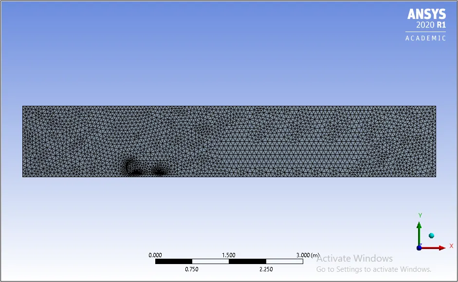
Fig. 2: Baseline Mesh

Mesh statistics and coefficient of drag values for Baseline Mesh:

Mesh	Element-Size(m)	Nodes	Elements	Coefficient of Drag(Cd)
Baseline	0.075	35354	177696	0.41846

Table 17: Mesh statistics and coefficient of drag values for Baseline mesh of the bluff body

Mesh quality attributes for Baseline Mesh:

Mesh	Element Quality(avg.)	Aspect Ratio(avg.)	Skewness(avg.)	Orthogonal Quality(avg.)
Baseline	0.83328	Triangles - 1.8613	0.23376	0.7649

Table 18: Mesh quality attributes depicting the average values of element quality, aspect ratio, skewness and orthogonal quality for Baseline mesh of the bluff body

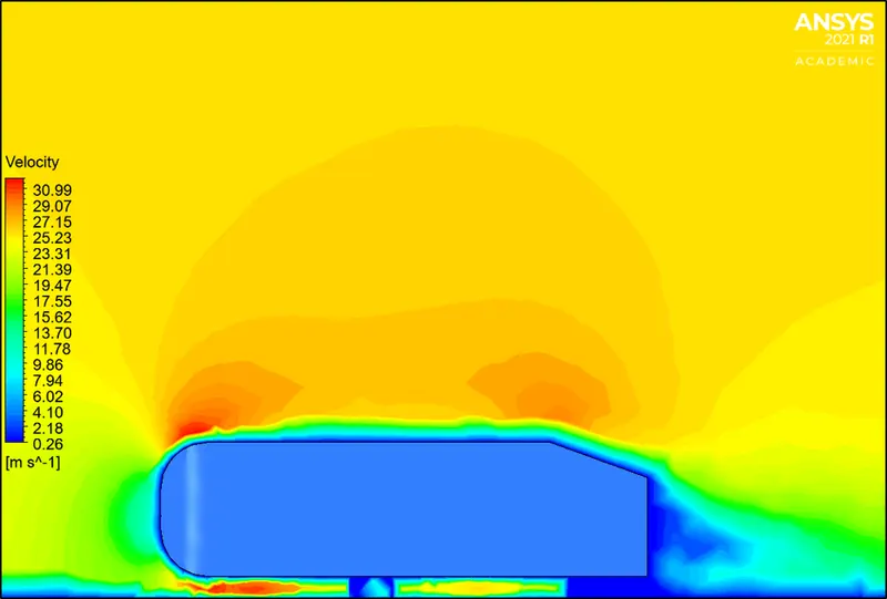
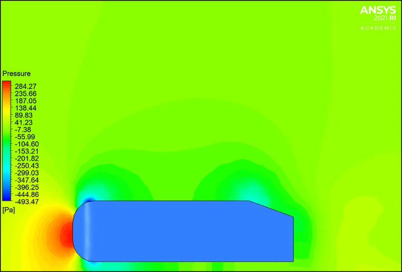
Fig. 3: Velocity and Pressure contour plot for Baseline Mesh at Isosurface 1

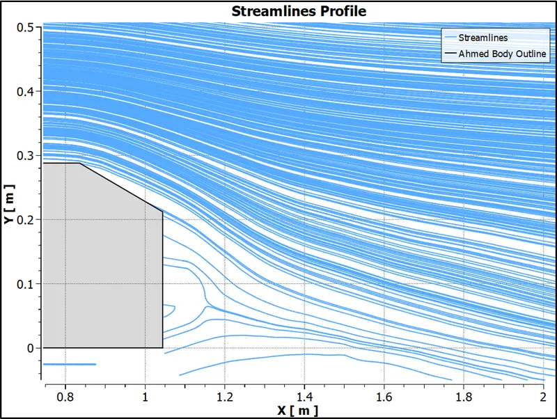
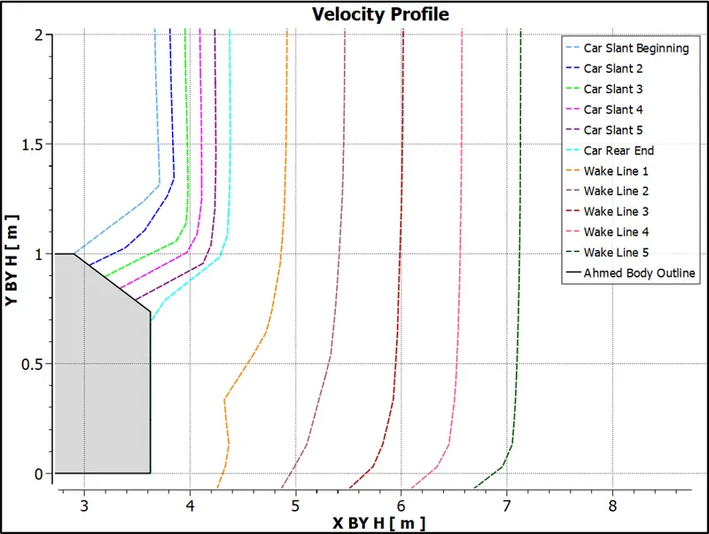
Fig. 4: Streamlines Profile and Velocity Profile (normalised using height of given Ahmed Body model) for Baseline Mesh at Isosurface 1

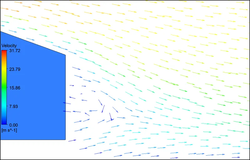
Fig. 5: Vector Plot for Baseline Mesh at Isosurface 1

Section 2.5.2 Mesh Refinement approach

The initial results obtained from the Baseline mesh in Section 2.5.1 Baseline Mesh both from Fig. 3 Velocity and Pressure contour plot for Baseline Mesh at Isosurface 1 and Fig. 4 Streamline Profile and Velocity Profile (normalised using height of given Ahmed Body model) for Baseline Mesh at Isosurface 1, indicated a significantly stronger presence of the recirculation region behind the vehicle body upto a distance of 0.8001m, fluid imposing region at a distance of 0.32004m in front of the vehicle body wherein the velocity profile begins to change, height from the ground (bottom surface of the computational domain) at 0.8001m within which the velocity and pressure gradient is large while the width from the symmetry plane towards the back surface of the computational domain as 0.40005m for the same. It should be noted that the values shown in the legend in Fig. 3 are with regards to the local plot variable values. Based on these dimensional extents from preliminary analysis, a refinement box was created in SpaceClaim by following steps similar to the creation of the computational domain. The mesh refinement hereafter was created while adhering to the mesh quality attributes mentioned in Section 2.2 Meshing. The region between the refinement box and the computational domain made use of the "MultiZone" method with "Mapped Mesh Type" as "Hexa" and "Surface Mesh Method" as "Program Controlled" since this area does not contain complex features, such as curves, thereby allows the meshing solver to implement the highest quality of cells i.e., "Hexa" cells, by identifying the different but fairly simplistic four edged surface combinations. Apart from the implementation of "Hexa" cells by using the "MultiZone" method, the cell count for the same element size reduces when compared against tetrahedral cells which in effect also improves the computational time. Within the refinement box and especially with regards to the Ahmed Body model, there exists many intricate surface features such as the cylindrical "stilts" (used for attaching the Ahmed Body to the ground i.e.., the bottom wall), the rounded "fore body" and the "slant" surface at the rear end of the vehicle, each of which requires an appropriate discretization approach. For the cylindrical "stilts", "Edge Sizing" was chosen to uniformly divide the meshing elements and to minimize errors due to numerical diffusion. The "Edge Sizing" type was selected as "Number of Divisions" and the value was set to 36 implying that the division was taking place at a point every 10° on the circle. The rounded "fore body" and the "slant" surface at the rear end of the vehicle were both initially discretised using the "Face Sizing" feature, however, due to the limitations in overall cell count to 512,000, it was decided to implement inflation layers instead which are required to capture the flow accurately around the Ahmed Body for prediction of coefficient of drag (Cd) values. Lastly, the region between the Ahmed Body and the refinement box was discretized using the "Body Sizing" feature which because of the relatively complex features of the former led to mesh creation of predominantly tetrahedral cells.

In order to add inflation layers, the boundary layer development for flow around the Ahmed Body and along the "bottom-wall" was required to be evaluated based on the governing conditions and flow properties which is shown below:

Reynolds number (based on model length):

`Re = (U*L*rho)/mu`, where (Eq. 1)

`U` is the freestream velocity,

`L` is the characteristic length, which in the case of the bluff body is its model length and for the "bottom-wall" is the length of the flat plate leading upto the bluff body,

`rho` is Density of fluid, and

`mu` is the dynamic viscosity of fluid

Since, the Reynolds number for the given flow conditions around Ahmed Body by substituting the given values in (Eq.1) equates to 1786772.102, it implies that the fluid flow lies in the turbulent flow regime. Also, based on experimental findings of Roshko (1954) on smooth cylinder and reported by C. H. K. Williamson [4], the boundary layer separation for external flow with regards to the evaluated Reynolds number is turbulent in nature.

To calculate the turbulent boundary layer thickness, we make use of the Prandtl's solution which can mathematically be expressed as:

`delta_L = 0.16*Re_x^(6/7)*(nu/U)`, where (Eq. 2)

`nu` is kinematic viscosity which is also equal to the ratio of dynamic viscosity to the density of the fluid flowing in the domain (`mu/rho`),

`Re_x` is the Reynolds number for the characteristic length, and

`U` is the freestream velocity

For Reynolds number evaluated from (Eq. 1), density value of 1.225 `(kg)/m^3` and the Viscosity (or dynamic viscosity) value of `1.7894*10^(-5) (kg)/(ms)`, the turbulent boundary layer thickness using Eq. 2 is determined to be 0.0214m for the Ahmed Body.

In order to capture the flow separation along the slant surface near the rear end of the bluff body and the resulting recirculation region near the wall, the approach adopted for evaluating the distance from the cell-centroid 'P' to the wall (`y_P`) and correspondingly the first cell height (`Delta_y`) was to target a `y^+` value such that the first grid cell would lie in the range of 30<`y^+`<300 for the RKE turbulence model so as to implement the wall modelling strategy for the log-law layer using the standard wall function approach. To ensure `y^+` value in the previously specified range, we need to calculate the values of wall shear stress and frictional velocity as shown below:

Wall Shear Stress:

`tau_w = (1/2)*C_f*rho*(U_(infty))^(2)`, where (Eq. 3)

`tau_w` is Wall shear stress,

`C_f` is Skin Friction coefficient,

`rho` is Density of fluid, and

`U_infty` is the freestream velocity

Skin Friction Coefficient (`C_f`) based on a semi-empirical expression can be related to the Reynolds number as shown below:

`C_f = 0.027/(Re_x)^(1/7)` (Eq. 4)

Frictional velocity (`U_tau`) can be computed mathematically as:

`U_tau = sqrt ((tau_w)/(rho))` (Eq. 5)

`y^(+)` is defined as the non-dimensional wall distance for a wall bounded flow that can be expressed mathematically as:

`y^+=(ρ*U_tau*y_P)/mu`; where (Eq. 6)

`y_P` is distance from the cell-centroid 'P' to the wall such that `Delta_y = 2*y_P`.

Simplifying (Eq. 6) to determine First Cell Height (`Delta_y`), we get;

`Delta_y = 2*(y^(+)*mu)/(rho*U_tau)` (Eq. 7)

Similarly, repeating the calculations for the boundary layer thickness development on the ground ("bottom-wall") as a result of the 'no-slip' boundary condition, we obtain a Reynolds number of 3573544.205 and a turbulent boundary layer thickness of 0.0387m. For Reynolds number of 1786772.102 and 3573544.205 representing the Ahmed Body and ground boundaries respectively with dynamic viscosity value of `1.7894*10^(-5) (kg)/(ms)`, density value of 1.225 `(kg)/m^3`, free-stream velocity values of 25m/s and `y^(+)` value of 150, the skin-friction coefficient (`C_f`), wall shear stress (`tau_w`), friction velocity (`U_tau`) and eventually the first cell height (`Delta_y`) values using (Eq. 4), (Eq. 3), (Eq. 5) and (Eq. 7) respectively are calculated in the following table:

Reynolds Number	Skin-friction Coefficient (`C_f`)	Wall Shear Stress (`tau_w`)[kg m^-1 s^-2]	Friction Velocity (`U_tau`) [m s^-1]	First Cell Height (`Delta_y`) [m]
1786772.102	`3.453*10^(-3)`	1.322	1.039	`4.2177*10^(-3)`
3573544.205	`3.128*10^(-3)`	1.197	0.988	`4.4354*10^(-3)`

Table 19: Skin-friction coefficient, wall shear stress, friction velocity and first cell height values for the governing flow conditions of the Ahmed Body

Calculation of Inflation Layers based on First Cell Height (`Delta_y`) and Turbulent Boundary Layer Thickness (`delta_L`):

From ANSYS Meshing User's Guide, the default growth rate type for determining height of inflation layers is Geometric. By mathematical formulation, the total height at layer 'n' for geometric growth rate type can be given by:

`H = h*((1-r^n))/((1-r))`, where (Eq. 8)

H = Total Height at layer 'n' i.e., Turbulent boundary layer thickness (`delta_L`),

r = height ratio = 1.2,

h = Initial height = First Cell Height i.e., `Delta_y`, and

n = Layer number

The missing variable in (Eq. 8) is n, or in this case total number of inflation layers. Equating for n in (Eq. 8), we get total number of inflation layers as a round figure value of 4 on the Ahmed Body and 6 for the ground boundary. Based on values obtained with regards to turbulent boundary layer thickness and number of inflation layers, four different meshes were prepared to identify the mesh independent solution, the details for which are reported in Table 20.

Mesh	Turbulent Boundary Layer Thickness on Car [m]	Body Sizing Element Size [m]	% increase in element size (w.r.t Turbulent Boundary Layer Thickness on Car)	Mesh Element Size [m]	% increase in element size (w.r.t Body Sizing Element Size)
1	0.0214	0.03638	70	0.06185	70
2	0.0214	0.03424	60	0.05478	60
3	0.0214	0.0321	50	0.04815	50
4	0.0214	0.031351	46.5	0.04593	46.5

Table 20: Body Sizing Element Size and Mesh Element Size for different meshes of the bluff body with regards to Turbulent Boundary Layer Thickness on Car

Mesh 1:

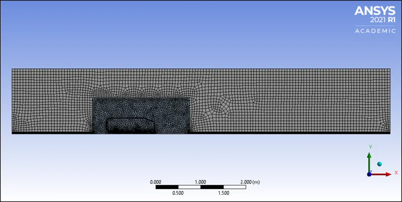
Fig. 6: Mesh 1

Mesh 2:

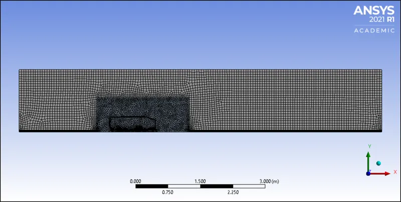
Fig. 7: Mesh 2

Mesh 3:

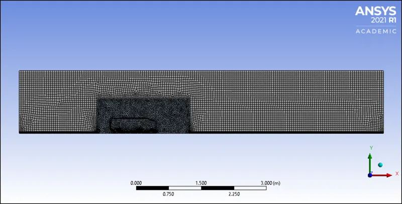
Fig. 8: Mesh 3

Mesh 4:

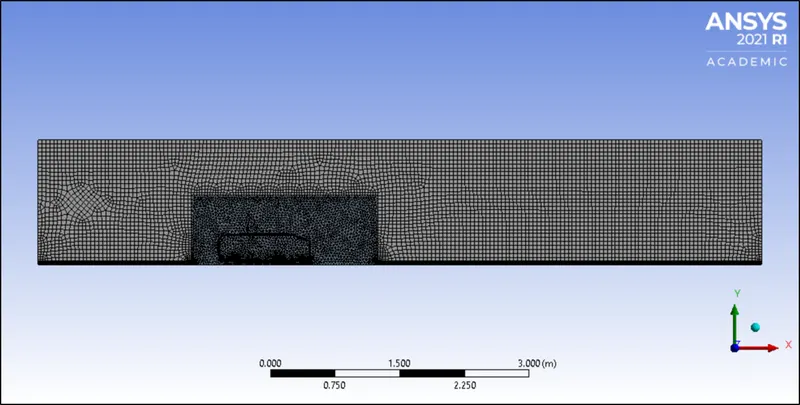
Fig. 9: Mesh 4

Mesh statistics and coefficient of drag values for the four different meshes:

Mesh	Nodes	Elements	Coefficient of Drag (Cd)	% var
1	183415	323995	0.35051	--
2	232131	389516	0.34312	-2.1083
3	284918	462644	0.34487	0.51
4	318117	509129	0.34393	-0.2726

Table 21: Mesh statistics and coefficient of drag values for different meshes of the bluff body

Mesh quality attributes for the four different meshes:

Mesh	Element Quality(avg.)	Aspect Ratio(avg.)	Skewness(avg.)	Orthogonal Quality(avg.)
1	0.75478	Triangles and Quadrilaterals - 2.6664	0.16319	0.84509
2	0.78724	Triangles and Quadrilaterals - 2.4344	0.15032	0.85762
3	0.78817	Triangles and Quadrilaterals - 2.3483	0.1393	0.86832
4	0.79483	Triangles and Quadrilaterals - 2.2881	0.13717	0.87187

Table 22: Mesh quality attributes depicting the average values of element quality, aspect ratio, skewness and orthogonal quality for the four different meshes of the bluff body

From the meshing statistics in Table 21, mesh number 3 (or mesh 3) with Body Sizing element size of 0.0321m and Mesh Element Size of 0.04815m represents a mesh independent result in terms of minimum percentage variation (%var) of the coefficient of drag values. The %var is calculated as the ratio of the difference of the predicted values in two consecutive meshes to the predicted value of the previous mesh e.g., ((Coefficient of drag for Mesh 2 - Coefficient of drag for Mesh 1)/Coefficient of drag for Mesh 1). Also, the quality attributes of all four meshes in Table 22 indicate that they all lie in the range of 'good' to 'very good' scale, when compared against Table 1, with each consequent refined mesh only improving the overall quality of the same. Due to constraints in computational resources and limitations in maximum number of cells/nodes for solution by ANSYS Student license to 512,000 any further reduction in Body Sizing element size and Mesh element size was not possible to achieve for the given numerical analysis. Results in Section 3 will only be referred with regards to the mesh independent solution i.e., Mesh 3.

2.5.3 Convergence Level

In the given numerical analysis, we are performing a steady-steady simulation using a Pressure based solver due to the low Mach number as specified in Section 2.3.3 Solution. For the given numerical analysis, three different schemes viz., SIMPLE, SIMPLEC and COUPLED, were compared to understand the effect on convergence and stability of coefficient of drag plots as they are preferred algorithms for solving steady-state numerical problems unlike PISO which is generally used for transient calculations with large time steps. SIMPLE scheme is iterative in nature, robust (memory efficient) and is quicker per iteration than other pressure-based solvers. SIMPLEC scheme, similar to the SIMPLE scheme, allows increased under relaxation to the pressure correction term that improves in convergence times especially when employed in complicated flows with turbulence and/or supplementary physical models and as such offers greater diversity in terms of computational problems for implementation over SIMPLE scheme. While SIMPLE and SIMPLEC schemes are segregated type of schemes i.e., pressure and velocity terms are updated sequentially, the COUPLED scheme on the other hand updates the pressure and velocity terms simultaneously. This allows the COUPLED scheme to be more efficient in its single phase implementation especially for steady-state flows offering superior performance over the segregated algorithms (SIMPLE and SIMPLEC) thereby requiring fewer iterations to converge. The selection of schemes for the different terms under spatial discretization includes assigning Gradient to Least Squares Cell Based scheme, pressure to second order scheme, momentum to second order upwind scheme, Turbulent Kinetic Energy to first order upwind scheme and Turbulent Dissipation Rate to first order upwind scheme of which the Turbulent Kinetic Energy and Turbulent Dissipation Rate. Least Squares Cell Based scheme is the default gradient method chosen by ANSYS Fluent which is used to compute the change in values across the centroid of two cells along a vector path and is a computationally less expensive scheme offering comparable accuracy to the node-based gradient scheme, both of which are superior to the cell-based gradient scheme. The second order scheme for the pressure makes use of the central differencing scheme and is generally considered to be more accurate than the Standard and Linear schemes as well as robust in the case of skewed meshes. A second order upwind scheme is chosen for the momentum and energy terms that makes use of the quantities at the cell face values to compute a cell-centered solution at the cell centroid leading to a second order accurate solution. The turbulence terms viz., Turbulent Kinetic Energy and Turbulent Dissipation Rate are set at first order upwind scheme by default which makes use of quantities at the cell faces as the cell-average value indicating that it is first-order accurate. The reason to have the turbulence terms discretized using the first-order upwind scheme is based on observations from simulations across different applications when using a higher or even second order upwind scheme leads the computational cost to become more expensive (more compute time) solution while also demonstrating stability issues in the form of repeating oscillations of values and not necessarily guaranteeing always a more accurate solution. Convergence criteria option was checked off, however, the residual values which measures the local imbalance of conserved variable in each control volume such as continuity, x-velocity, y-velocity, k and `epsilon` were monitored throughout the solution process for the defined number of iterations to allow the actual fluid behaviour to be developed i.e., the formation of the wake and recirculation regions. The residual limits defined for the turbulence model equations and the residual plots corresponding to the different meshes are shown in the table and figures below:

	RKE
continuity	1e-03
x-velocity	1e-03
y-velocity	1e-03
z-velocity	1e-03
k	1e-03
epsilon	1e-03

Table 23: Residual Values of the different equations used in the RKE turbulence model

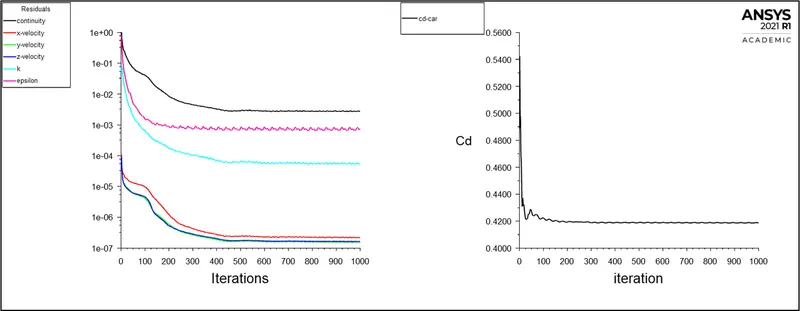Fig. 10: Scaled Residuals and Coefficient of Drag plots using the RKE turbulence model for baseline mesh with SIMPLE solver

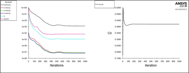Fig. 11: Scaled Residuals and Coefficient of Drag plots using the RKE turbulence model for baseline mesh with SIMPLEC solver

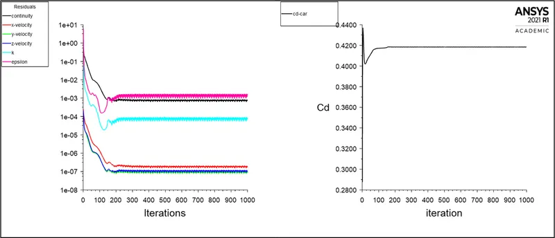Fig. 12: Scaled Residuals and Coefficient of Drag plots using the RKE turbulence model for baseline mesh with COUPLED solver

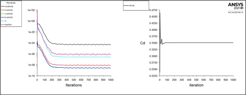Fig. 13: Scaled Residuals and Coefficient of Drag plots using the RKE turbulence model for mesh 1 with COUPLED solver

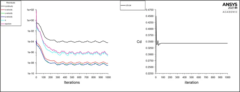Fig. 14: Scaled Residuals and Coefficient of Drag plots using the RKE turbulence model for mesh 2 with COUPLED solver

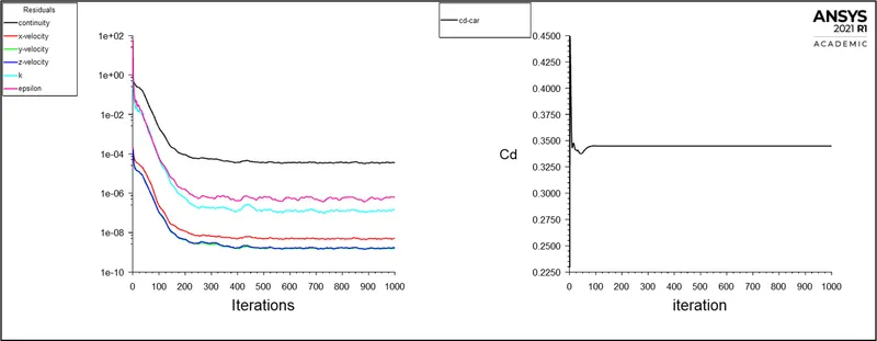Fig. 15: Scaled Residuals and Coefficient of Drag plots using the RKE turbulence model for mesh 3 with COUPLED solver

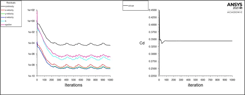Fig. 16: Scaled Residuals and Coefficient of Drag plots using the RKE turbulence model for mesh 4 with COUPLED solver

From Fig. 10, Fig. 11 and Fig. 12, we can notice that the residuals for SIMPLE and SIMPLEC scheme have not shown stable convergence and also are converging well above the '1e-03' default limit (although not being considered as the convergence criteria option was checked off) for continuity equation whereas for the COUPLED scheme, convergence based on the residual values mentioned in Table 27 and Coefficient of Drag plots shows a highly stable output well before they reach the total number of iterations indicating that a steady-state solution has been obtained. This reconfirms the expected behaviour from each of the schemes. Although, the time taken to achieve convergence using the COUPLED solver was more than the SIMPLE and SIMPLEC solvers, the results obtained made it more reliable and accurate for it to be reused to solve the pressure-velocity equations for the four different meshes that were prepared to obtain a mesh independent solution and later to be compared against experimental values.

3. Results

In Section 3.1, numerical simulation results for drag coefficient are compared against experimental values referenced in both [1] and [2] while in Section 3.2, velocity and static pressure contour, streamline and vector plots to demonstrate the development of velocity and static pressure profiles as well as the wake region behind the bluff body with regards to the mesh independent solution are discussed.

3.1. Validation of numerical results against experimental values for drag coefficient

Fig. 15 shows the Scaled Residuals and Coefficient of Drag plots for the mesh independent solution of which the coefficient of drag has a computed value of 0.34487. It can be seen from Table 24 that the numerically computed value overpredicts the experimental drag coefficient by 4.506%. The difference in the computed values and experimental value for drag coefficient can be attributed to the computational constraints and meshing restrictions as mentioned in Section 2.5.2 Mesh Refinement approach. The other reason for discrepancy in predicted values using numerical analysis can be related to the behaviour of vortices generated in the wake and the flow separation phenomena which is in turn dependent on the value of the slant angle, discussed in detail in Section 4. Discussion, that the RKE turbulence model among many other turbulence models is not able to estimate correctly. However, even though the drag coefficient is overpredicted by the turbulence model used for this numerical analysis, the physical phenomena for the given configuration with regards to the recirculation region was replicated successfully as was observed in experimental studies [2].

Coefficient of Drag (Numerical Analysis vs Experimental Results):

Coefficient of Drag(Cd) - Numerical Analysis	Coefficient of Drag(Cd) - Experimental Results	Absolute Difference (%)
0.34487	0.33	4.506

Table 24: Comparison of Coefficient of Drag values between Numerical Analysis and Experimental Results for mesh independent solution of the bluff body

3.2 Wake region behind the Ahmed Body using velocity and static pressure contour plots, vector plots, streamline profile and velocity profile

Fig. 17, Fig. 19 and Fig. 18, shows the recirculation region behind the bluff body using velocity and static pressure contour plots, vector plots, and streamline and velocity profiles respectively. The static pressure contour plot highlights high pressure areas characterised towards the fore body region where the velocity values are low since the flow that is directed towards this area begins to move along the surface in an attached manner. The static pressure undergoes a massive drop when the geometry changes at sharp corners such as the transition from forebody to the mid-section and from the mid-section to the slant before leaving the vehicle body at the rear end as the velocity begins to accelerate in order for the fluid flowing across the bluff body to adhere to its surface which can also be seen in the velocity contour plot. Across the slant surface for the given configuration of the Ahmed Body, the flow that separates yet again (as seen in the velocity contour plot and streamlines profile) leads to a lowering of pressure levels (as identified by negative values with reference to the legend of the pressure contour plot) which because of the vortex mechanism involved, discussed in detail in Section 4. Discussion, causes the creation of a recirculatory region as can be seen in the streamlines profile plot. The velocity profiles and vector plots in Fig. 18 and Fig. 19 represented by inverted profile representation and cross flowing velocity vectors indicate the presence and length of the wake region beyond the bluff body.

For Mesh 3:

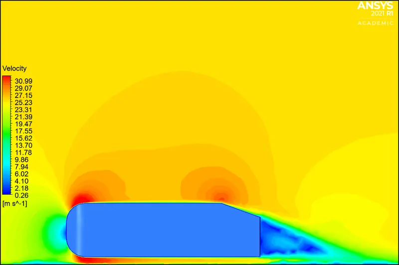
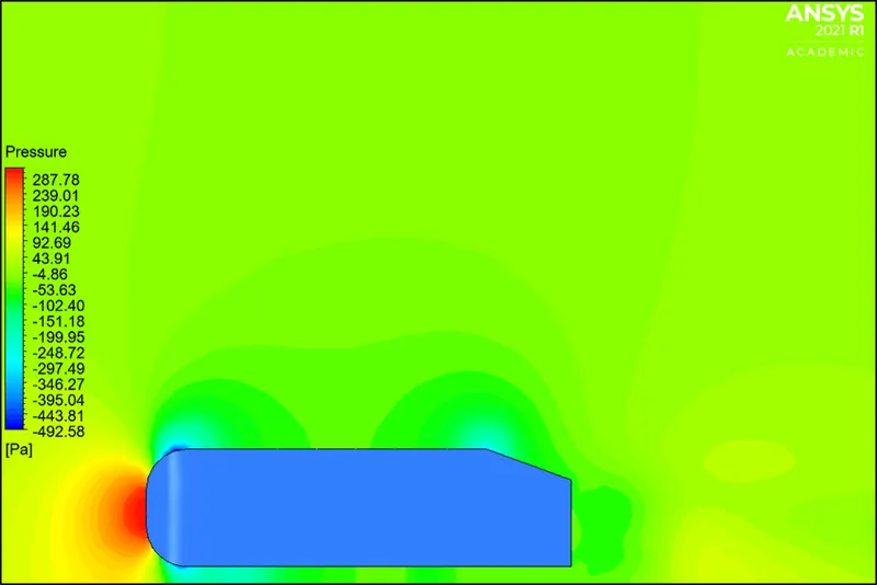Fig. 17: Velocity and Pressure contour plot for Mesh 3 at Isosurface 1

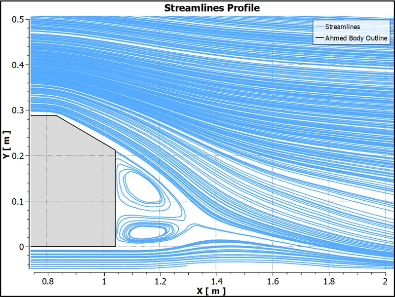
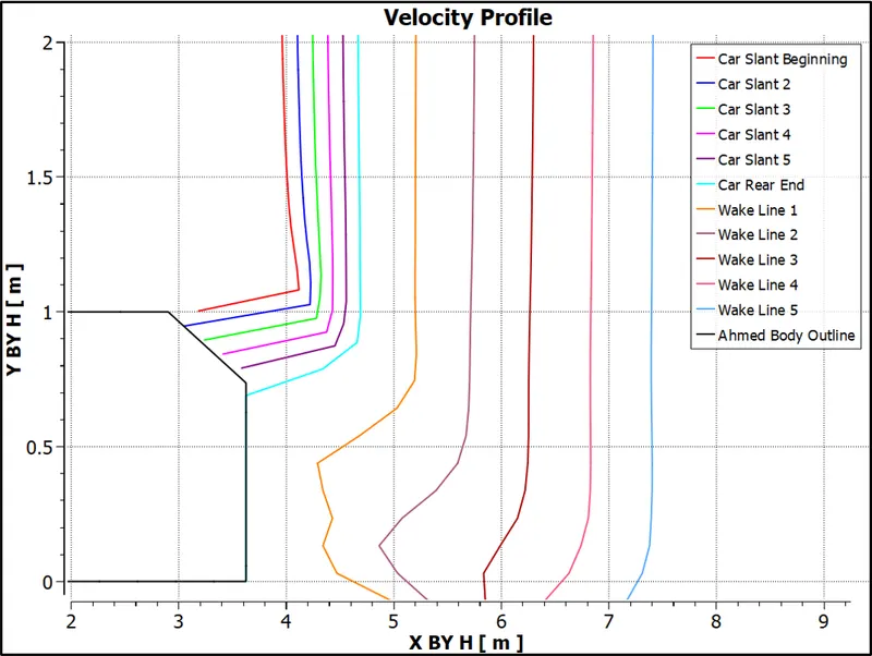Fig. 18: Streamlines Profile and Velocity Profile (normalised using height of given Ahmed Body model) for Mesh 3 at Isosurface 1

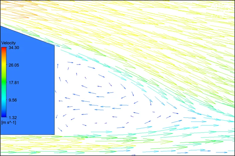
Fig. 19: Vector Plot for Mesh 3 at Isosurface 1

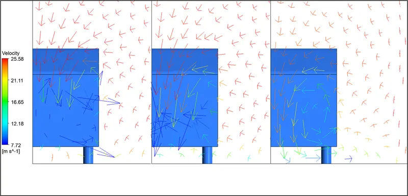
Fig. 20: Cross flow velocity distribution at three downstream stations (defined w.r.t planes in Tables 14, 15 and 16 subsequently) in the wake along the transverse direction

4. Discussion

The fluid flowing across the bluff body begins to split at the forebody region due to the rounded shape leading to decrease in the flow velocity and a subsequent increase in pressure. Depending on the governing flow conditions, a flow separation and recirculation region can be observed on the forebody region, however, these features were not observed based on the testing conditions in experimental studies [2] in reference. The flow begins to move along the surface due to the continuous fluid motion until the sudden change in geometry is encountered towards the beginning of the mid-section of the bluff body. This leads to a separation of the fluid experienced by low pressure values and the fluid accelerates to reattach itself to the vehicle body. This separation and subsequent reattachment gives rise to longitudinal vortices further downstream along the mid-section of the body which is characteristic of the attached turbulent boundary layer. As the flow approaches the slant edge of the bluff body, the characteristics become complex and are mostly dictated by the slant angle value. For the given configuration, it is observed from detailed near wake measurements in [2], that a small recirculation region is formed in the upper part of the slant, however, beyond this region the flow reattaches to the slant surface before forming a second and larger recirculation region along the lowermost part of the rear end of the bluff body. This is because streamwise counter-rotating vortices are generated at the slant edges in lateral direction as the flow along the mid-section of the body is pulled into the low pressure region immediately above the slant by virtue of the presence of a strong pressure gradient. The shear layer begins to come off the slant edge as the flow approaches the rear end of the vehicle and eventually splits to form two recirculatory regions due to the rolling up of the longitudinal vortex. As the flow progresses downstream, the upper recirculatory region merges with the flow that is separated from the transition point at the top surface and the slant as can be seen in Fig. 20 with the cross flow velocity distribution at three downstream stations in the wake at transverse locations. The given bluff body configuration also has the presence of a side vortex and energy transfer to it takes place from the separation bubble as was observed in [1], however, the same was not identified by the turbulence model chosen for this study as the point or size of separation zone was not estimated on the slant surface and instead the RKE turbulence model assumes the flow is still attached. The point of separation as such impacts the topology of the flow structures in the wake especially for the given configuration wherein the presence of a strong side edge vortex is absorbing the low energy from the separated flow region as well as the subsequent lowering of pressure values leading to an increase in the pressure drag, a component contributing to the overall drag on the vehicle.

5.Conclusion

The numerical analysis for flow over Ahmed Body under steady state conditions using the RKE turbulence model in ANSYS Fluent 2021 R1 was well understood. It was realised that based on the boundary layer development over the Ahmed Body and use of an appropriate viscous model, a CFD model was able to replicate the wake region beyond the vehicle body. Additionally, the recirculatory regions observed gave a deeper understanding of the flow regime with regards to the Ahmed Body configuration and demonstrated the capabilities of this mathematical model when validated against experimental results. However, the RKE turbulence model used for this simulation failed to predict the point of separation, the separation region and the reattachment on the slant surface which from several numerical simulation studies by different authors lead to a consensus that turbulence models are sensitive to the geometry of the bluff body and the fluid mechanical behaviour for the same. Also, the overall drag coefficient predicted for the given configuration could achieve better correlation with an improved mesh refinement across the computational domain.

References

[1] S.R. Ahmed, G. Ramm, Some Salient Features of the Time-Averaged Ground Vehicle Wake, SAE-Paper 840300, 1984

[2] H. Lienhart, C. Stoots, S. Becker, Flow and Turbulence Structures in the Wake of a Simplified Car Model (Ahmed Model), DGLR Fach Symp. der AG STAB, Universität Stuttgart, November 15–17

[3] R. Manceau, J. Bonnet, eds., 10th joint ERCOFTAC/IAHR/QNET-CFD Workshop on Refined Turbulence Modelling, Poitiers, France 2002

[4] C. H. K. Williamson, VORTEX DYNAMICS IN THE CYLINDER WAKE, Annual Review Fluid. Mech., 1996