Conjugate Heat Transfer Analysis on a graphics card.

1. Introduction

Processes involving interaction of thermal energy between a solid body and fluid volume at interfaces common to both domains leading to forming a thermally coupled system can be described as conjugate heat transfer (CHT) phenomena. CHT analysis for a coupled system takes into account the physical processes and governing equations occurring within the individual subdomains as separate entities and then evaluates the heat exchange based on those local variations at the interfaces, depending on the boundary conditions, to get the requisite temperature and heat flux distribution thereby avoiding the need of separate empirical relations. Therefore, a CHT analysis offers the advantages of observing and recording both fluid flow and heat transfer changes and calculation of wall heat transfer coefficient, temperature and velocity profiles across the domain in real time. Applications of CHT analysis include, but are not limited to, development of exhaust port system in automotive and commercial vehicles, designing of energy saving applications such as thermal insulators in windows by using gases (not in motion) with solids to limit loss of heat by natural convection especially in regions that experience extremely low temperatures. In recent years and with advancements in consumer electronics, CHT analysis has become extremely important in assessing the cooling performance of systems, such as the commonly used heat sinks, in order to predict the effectiveness of its design, feasibility and viability across different thermal and physical conditions for both the electronic components and cooling systems as they would be subjected to in real-world scenarios.

The aim of this challenge is to perform steady-state simulations at 3 input velocities between 1m/s and 5m/s, in this case being 1m/s, 2.5m/s and 5m/s respectively, to understand the velocity and temperature profiles development within the enclosed domain that would influence the maximum temperature and heat transfer coefficient attained by the processor as well as identification of potential hotspots on the model. The graphics card is an expansion card containing an assembly of various electronic components that perform computations to generate series of images rendered on a display device, like a monitor, outputted to it in the form of electrical signals. At the heart of it, the graphics card contains the processor (also known as graphics processing unit or GPU), with the other electronic components typically connected on a printed circuit board (PCB) that is placed into an expansion slot which can be either integrated onto the motherboard of a computing system or installed as a supplementary component depending on the configuration of the same. The given graphics card model consists of the processor, PCB as the base for all electrical connections, heat sink for cooling in the form of an array of aluminium fins, capacitors and memory card as the electronic components and the support bracket for mounting the graphics card component to the chassis of the computing system. The analysis involves verification of the computed results with a mesh independence study detailing on the mesh refinement approach based on a combination of coarse and refined mesh in different regions which would also outline cell count, maximum temperature and average wall heat transfer coefficient values obtained by the processor and number of iterations for convergence for each mesh based on stability of behaviour of maximum temperature and average wall heat transfer coefficient values as well as some of the mesh quality attributes like element quality, skewness, orthogonality and aspect ratio.

2. Method

2.1 Modelling

The given graphics card configuration was modelled in SpaceClaim, the default solid modeling CAD software for the Fluid Flow (Fluent) Analysis System. Since, the graphics card model has different electronic components that are placed unequally along the flow axial direction and a non-symmetrical structural design for the support bracket such that the heat transfer contribution from all the associated parts influences the output thermal properties of the processor despite having isothermal boundary conditions and uniform input flow of constant magnitude in all directions defined in a three-dimensional space, the simulations cannot be carried out for one half of the model i.e., the model size cannot be reduced for a faster computational time. Therefore, the entire model needs to be utilised for discretization and solution of the partial differential equations which will be discussed in detail regarding the setup in subsequent sections. As both the solid bodies and the Fluid Volume will be required for discretization for evaluating average wall heat transfer coefficient by the processor due to the nature of the simulation i.e., CHT analysis, it is important to ensure that the nodes along the interfaces in the mesh match, or in other words is conformal, which also reduces interpolation to a minimum, improves computational time and renders higher accuracy to the solution. For obtaining the conformal mesh, allowing exchange of information during the solution process owing to the fluid-solid interactions and avoiding failure to create mesh during the meshing process, the 'Share' option in both 'Share Topology' under the 'Properties' window in the parent link of the design/model structure tree and in 'Sharing' section under the 'Workbench' tab respectively was enabled.

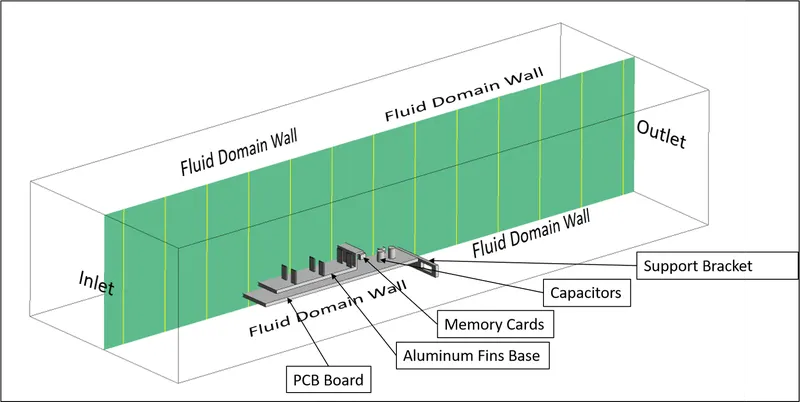
Fig. 1: Solid Bodies, Fluid Volume Models and Boundary Conditions regions (processor between aluminium fins base and PCB Board)

2.2 Meshing

The meshing approach adopted for the given computational domain was developed to maintain the meshing quality attributes viz., element quality, skewness, orthogonality and aspect ratio within the ranges as laid out in the Meshing training material of ANSYS outlined in the following table:

Element Quality			0 (Bad Mesh)	1 (Good Mesh)
Aspect Ratio		Triangles	1 (for an equilateral triangle)	- Best possible value
		Quadrilaterals	1 (for a square)	- Best possible value
Skewness	0-0.25 (Excellent)	0.25-0.50 (Very Good)	0.50-0.80 (Good)	0.80-0.94 (Acceptable)	0.95-0.97 (Bad)	0.98-1.00 (Unacceptable)
Orthogonal Quality	0-0.001 (Unacceptable)	0.001-0.14 (Bad)	0.15-0.20 (Acceptable)	0.20-0.69 (Good)	0.70-0.95 (Very Good)	0.95-1.00 (Excellent)

Table 1: Mesh Quality Attributes as defined in the ANSYS meshing training material

The reason for targeting the above-mentioned mesh quality attributes comes from analysis across different types of geometries/models that these are few of the known ways of identifying whether the discretized mesh would develop convergence issues during the solution process and also to locate areas in the mesh where the statistics can be improved. For each of the mesh, named selections such as inlet, outlet and walls for the fluid domain, and component related walls for the solid domains have been created so as to assign their respective boundary conditions in the setup stage. The shared interface between the solid and fluid domains is detected by the Fluent solver as the region of coupled thermal condition since exchange of heat transfer takes place along this boundary further highlighting the importance of conjugate heat transfer analysis. Also, depending on the name of the named selection, Fluent is able to assign inlet, outlet, and wall boundary conditions with velocity-inlet, pressure-outlet, and coupled wall type boundary conditions respectively which is a useful feature to have in flow-type problems of similar nature since the user now can only add values relating to the specific boundary condition thereby making the setup process a lot faster. In Section 2.5.2, we will discuss in detail about the different meshes that were prepared, their mesh qualities and the arrival on mesh independent solution based on a combination of coarse and refined mesh in different regions.

2.3 CFD Simulation Setup, Boundary Conditions, Monitoring Points and Solution

The simulations on all meshes was performed using the Laminar viscous model as the Reynolds number, based on the input flow conditions and characteristic length of the processor, represented fluid flow in the laminar regime when compared against equivalent Reynolds number for external flow over flat plate. Additionally, all simulations are being run using the double-precision feature to accurately measure the prediction quantities (maximum temperature) and as a general measure to resolve large variations in pressure differences. A brief description into the working of the laminar viscous model is provided below:

2.3.1 Laminar viscous model

The Laminar viscous model can be described as the solution of the governing fluid equation viz., Navier-Stokes equations for a domain, in this case, discretized using the finite volume approach, without the presence of turbulence terms. The Navier-Stokes equations define the fluid flow properties such as velocity, pressure, density, temperature, viscosity, energy, etc., within a given physical domain. Additionally, the Navier-Stokes equations are developed with regards to the laws of conservation that states the net mass flow across a system is zero (Conservation of mass), momentum within the same system (or control volume) is constant (Conservation of momentum) and since, energy is also a variable of assessment for the given domain, then according to the first law of thermodynamics, total heat gain of a system is equal to the sum of heat added to the system and work done on the same system.

2.3.1.1 Setup of the Laminar viscous model:

To use the Laminar viscous model in the Fluent component system, we navigate to Viscous option in Models under the Physics Tab. In the Viscous Model feature window, we choose Laminar as the option.

2.3.2 Boundary Conditions and Monitoring Points

The different boundary conditions for the CHT analysis on a graphics card is described in the following table:

Named Selections	inlet	fluid_domain_walls	heat_transfer_coefficient_capacitor_walls, heat_transfer_coefficient_fins_base_walls, heat_transfer_coefficient_memory_card_walls, heat_transfer_coefficient_pcb_base_walls, heat_transfer_coefficient_processor_walls, heat_transfer_coefficient_support_bracket_walls	outlet
Type	Velocity-inlet	wall	wall	pressure-outlet
Shadow Face Zone	--	--	heat_transfer_coefficient_capacitor_walls-shadow, heat_transfer_coefficient_fins_base_walls-shadow, heat_transfer_coefficient_memory_card_walls-shadow, heat_transfer_coefficient_pcb_base_walls-shadow, heat_transfer_coefficient_processor_walls-shadow, heat_transfer_coefficient_support_bracket_walls-shadow	--
Velocity Specification Method	Magnitude, Normal to Boundary	--	--	--
Velocity Magnitude (`m s^-1`)	1 2.5 5	--	--	--
Temperature (K)	300	--	--	--
Thermal Conditions	--	Heat Flux	Coupled	--
Wall Thickness (m)	--	0	0	--
Heat Generation Rate (`W m^-3`)	--	0	0	--
Heat Transfer Coefficient (`W m^2 K^-1`)	--	--	--	--
Heat Flux (`W m^-2`)	--	0	--	--
Gauge Pressure (Pa)	--	--	--	0
Wall Motion	--	--	--	--
Shear Condition	--	--	--	--

Table 2: Boundary Conditions for CHT analysis on the given graphics card model

For the given problem, the material properties can be summarised in the following table with the appropriate values of Density, Specific Heat and Thermal Conductivity for both solid domains and fluid domain and Viscosity (or dynamic viscosity) value for the fluid domain:

Domains/Cell Zone	Material	Density (`(kg)/(m^3)`)	Specific Heat (`J/(kg-K)`)	Thermal Conductivity (`W/(m-K)`)	Viscosity (`(kg)/(m-s)`)
Processor (Solid)	Silicon [1,4]	2330	707	170	--
PCB Base (Solid)	PCB [4]	2157	1117	20	--
Fins Base (Solid)	Aluminium [1]	2719	871	202.4	--
Capacitors (Solid)	Tantalum [1,3]	16650	140	57.5	--
Memory Cards (Solid)	Flame-retardant composite (FR4) [2,4]	1900	1200	0.23	--
Support Bracket (Solid)	Aluminium-alloy [5]	2096.5	1643.319	212	--
Enclosure (Fluid)	Air	1.225	1006.43	0.0242	`1.7894*10^(−5)`

Table 3: Material selection for different components on the given graphics card model

Since, the material properties are different from the standard and available materials in the Fluent database, new material definitions were created by heading over to the 'Materials' section of the 'Physics' tab and clicking on the 'Create/Edit' button. To create new materials mentioned in Table 3 in the 'Create/Edit Materials' window, we select 'solid' material type with 'aluminium' as the base material from the 'Fluent Fluid Materials' drop down menu, enter the name of the material followed by its physical and thermal property values under the appropriate headings before clicking on the 'Change/Create' button and selecting 'No' to not only ensure that the newly created material name and properties are saved as a copy but to also avoid overriding the properties of the base material, in this case, aluminium. In order to assign the newly created materials, we need to select the 'Cell Zones' option under the 'Zones' section of the 'Physics' Tab which also represents the named selections created during the meshing stage. After the appropriate zone has been highlighted in the 'Cell Zone Conditions' window, the 'Edit' button can be clicked on and the material created for that particular zone can be selected from the 'Material Name' drop-down list followed by clicking on the 'OK' button. In the case of the processor cell zone, volumetric heat source of 53333333.33 `W/(m^3)` is applied, which equates to about 150W of heat dissipation per volume of the processor equivalent to the Thermal Design Power (TDP) of a NVIDIA GeForce GTX 1070 GPU [6], by enabling the 'Source Terms' option in the selected cell zone window and heading over to the 'Source Terms' tab, editing the 'Energy' option to 1 source and entering the calculated value as a constant. It should be noted that a typical internal construction of a PCB is essentially multi-layered consisting of copper and glass fiber in the form of FR4, placed alternatively with varying thickness, with effective thermal conductivity for the given computational problem reflecting that of an average 4 copper conduction layers so as to assume isotropic material properties. To ensure the materials are also reflecting in the boundary conditions of the adjacent cell zones they belong to, the 'Boundaries' option under the same section as that of the 'Cell Zones' are selected and by clicking on the 'Edit' button of each boundary condition, the corresponding 'Material Name' can be changed or confirmed.

During the solution process, we are interested in monitoring the maximum temperature plot attained by the processor to observe stability in output of the predicted value. To create the required monitoring plot, we head over to the 'Definitions' drop-down menu in the 'Reports' section of the 'Solution' tab and choose 'Volume Average' option in the 'Volume Report' followed by assigning the name as volume-average-temperature, choosing 'Temperature' as the Field Variable and 'Static Temperature' as the attribute, selecting 'processor' in the 'Cell Zones' list, checking the 'Report File' and 'Report Plot' boxes before clicking on the 'OK' button. Fig. 1 outlines the named selections where the boundary conditions would be employed as well as contour plots to demonstrate the temperature distribution discussed in Section 2.3.3 Solution and Section 2.4 Post-Processing respectively.

2.3.3 Solution

The nature of the given CFD simulation is steady-state while the type of solver chosen is Pressure-based solver as we are dealing with a low-speed incompressible flow problem i.e., the speed of the fluid flow is typically in the subsonic range and the density of the material does not change or the change is almost negligible within the given control volume, although the Fluent Theory Guide also claims that the Pressure-based solver can now solve and operate beyond its previous limitations. The Pressure-based solver calculates the Pressure field by evaluating the pressure or pressure-correction equation that is determined from the manipulation of continuity and momentum equations. Velocity formulation is chosen to be absolute as the velocity in the given fluid control volume is not rotating. Before we run the solution, we need to initialise the given fluid volume which in this case is done using the Hybrid Initialisation option. Hybrid Initialisation as described in the Fluent Theory Guide solves a Laplace equation to create a velocity flow field that will adhere to the domain geometry and a pressure field across the same domain to allow smooth transition of high and low pressure values. A contour plot to depict the development of temperature gradient across the graphics card model during the simulation run and recorded as a MPEG animation file was setup. The contour plot was now available to be created under the 'Graphics' section of the 'Results' tab since the solution was initialized. After a new contour plot option has been selected from the 'Contours' drop-down menu, a name can be assigned, in this case, 'temperature-contour', followed by clicking on the 'Filled' check-box, choosing 'Temperature' as the field variable with 'Static Temperature' as the attribute and selecting all the surfaces representing the graphics card model and components in the 'Surfaces' list. We can now click on the 'Save/Display' button. To create an animation plot of the same contour, we can head back to the 'Solution' tab and click on the 'Solution Animations' option available under the 'Create' drop-down menu of the 'Activities' section. In the 'Animation Definition' window, we assign the name of the animation as 'Temperature' and choose 'temperature-contour' which is the name of the contour plot before clicking on 'OK'. Additionally, during the entire run, we will not be checking on the convergence criteria which can be disabled by selecting the 'Residuals' option in the 'Reports' section of the 'Solution' tab and unchecking the 'continuity', 'x-velocity', 'y-velocity', 'z-velocity' and 'energy' for laminar viscous model to monitor the solution based on the number of iterations.

2.4 Post-Processing

In order to plot the temperature contour plots and velocity vector plots across the enclosure model length for the given computational problem at different surfaces, Line and Plane locations at different positions within the fluid domain were drawn. Apart from the Line and Plane locations described in the tables below, expressions to calculate Reynolds number based on the input conditions and processor characteristic length, and temperature profiles in the direction of flow were created. Legends, titles, x and y labels have been added for temperature profiles, vector plots and contour plots for a better understanding of the graphical representation and can be viewed under Section 3 Results.

Expressions:

Maximum temperature (across the domain, in this case at the PCB base):

maximum temperature = maxVal(Temperature)@pcb_base

Temperature values against axial distance in the direction of flow normalised by model inlet diameter (h = 0.040505m):

x by h temp = (Temperature /(maximum temperature ) )*1[m] - (X/0.040505)

z-axial distance normalised by model inlet diameter (h = 0.040505m):

z by h = Z/0.040505

It is important to note that the first term on the right-hand side for the 'x by h temp' expression to evaluate normalised temperature values is actually a dimensionless number, however CFD Post does not recognise the same unless 'maximum temperature' is not multiplied by 1m, since it performs the addition of similar quantities only i.e., units on both sides of the '+' operator need to be in m.

Reynolds number calculation based on the processor length that represents the plan profile of the given cuboid as a square (as the horizontal dimensions parallel to the axial flow direction have edges of equal values):

L = 0.008 [m]

W = 0.008 [m]

H = 0.001 [m]

Aspect Ratio can be defined as:

AR = H/L

Characteristic length (based on a simplified analytical approach for forced convection heat transfer considering a cuboid model [7]):

L char = L * (2 * (AR + 1))^(1/2)

In order to determine average wall heat transfer coefficient at the processor based on the appropriate Nusselt number correlation for forced convection, average surface temperature at the processor walls need to be determined, in this case the walls that are exposed to the air flowing over it.

average surface temperature processor = ave(Temperature)@heat_transfer_coefficient_processor_walls.2

Properties of Air for evaluating Reynolds number and Prandtl number are evaluated at Film temperature which is defined as the mean of the wall and ambient temperature and is mathematically expressed as:

film temperature = (average surface temperature processor + ambient temperature)/2; where

ambient temperature = 300 [K]

Reynolds number based on characteristic length of the processor and kinematic viscosity evaluated at the film temperature can be expressed as:

Re L = (input vel * L char )/(kinematic viscosity of air at film temperature) (Eq. 1)

Similarly, Prandtl Number with values for dynamic viscosity, specific heat capacity and thermal conductivity of air evaluated at film temperature can be expressed as:

Pr = (dynamic viscosity of air at film temperature * specific heat capacity of air at film temperature)/thermal conductivity of air at film temperature (Eq. 2)

The resulting values of Reynolds number based on the characteristic length and different input velocities suggests that the resulting flow regime is laminar as can also be seen in Table 25. The Nusselt number correlation as a combined equation based on the local Nusselt number defined by Yovanovich et al [8] and use of square root of the surface area of the processor as the characteristic length by Lee et al. [9] in [7] can be mathematically expressed as:

Nu L char = (2/pi^(1/2))*(1/(((AR + 1)*C )/(2*(AR + 1))^(1/2))^(1/2))*(Re L )^(1/2)*(Pr )^(1/3); where (Eq. 3)

C = 2.5 (average between two extreme values for constant representing boundary layer parameter between high Prandtl number with heat flux representing exact solution of Pohlhausen and enthalpy heat flux across the thermal boundary layer for transient heat diffusion in half-space [7])

Average heat-transfer coefficient with regards to the Nusselt number correlation and characteristic length can be mathematically equated as:

average heat transfer coefficient processor = (Nu L char * thermal conductivity of air at film temperature )/L char (Eq. 4)

Definition of Lines at different distances along the spanwise flow direction (Refer Fig.1 indicated by yellow-coloured lines):

Line 1 @0.007m from the enclosure inlet:

Point	x[m]	y[m]	z[m]
Point 1	0.075	0	-0.0035
Point 2	0.075	0	0.037

Table 4: Definition of Line 1

Line 2 @0.022m from the enclosure inlet:

Point	x[m]	y[m]	z[m]
Point 1	0.06	0	-0.0035
Point 2	0.06	0	0.037

Table 5: Definition of Line 2

Line 3 @0.037m from the enclosure inlet:

Point	x[m]	y[m]	z[m]
Point 1	0.045	0	-0.0035
Point 2	0.045	0	0.037

Table 6: Definition of Line 3

Line 4 @0.052m from the enclosure inlet:

Point	x[m]	y[m]	z[m]
Point 1	0.03	0	-0.0035
Point 2	0.03	0	0.037

Table 7: Definition of Line 4

Line 5 @0.067m from the enclosure inlet:

Point	x[m]	y[m]	z[m]
Point 1	0.015	0	-0.0035
Point 2	0.015	0	0.037

Table 8: Definition of Line 5

Line 6 @0.082m from the enclosure inlet:

Point	x[m]	y[m]	z[m]
Point 1	0	0	-0.0035
Point 2	0	0	0.037

Table 9: Definition of Line 6

Line 7 @0.097m from the enclosure inlet:

Point	x[m]	y[m]	z[m]
Point 1	-0.015	0	-0.0035
Point 2	-0.015	0	0.037

Table 10: Definition of Line 7

Line 8 @0.112m from the enclosure inlet:

Point	x[m]	y[m]	z[m]
Point 1	-0.03	0	-0.0035
Point 2	-0.03	0	0.037

Table 11: Definition of Line 8

Line 9 @0.127m from the enclosure inlet:

Point	x[m]	y[m]	z[m]
Point 1	-0.045	0	-0.0035
Point 2	-0.045	0	0.037

Table 12: Definition of Line 9

Line 10 @0.142m from pipe Inlet downstream:

Point	x[m]	y[m]	z[m]
Point 1	-0.06	0	-0.0035
Point 2	-0.06	0	0.037

Table 13: Definition of Line 10

Line 11 @0.157m from pipe Inlet downstream:

Point	x[m]	y[m]	z[m]
Point 1	-0.075	0	-0.0035
Point 2	-0.075	0	0.037

Table 14: Definition of Line 11

Line 12 @0.172m from pipe Inlet downstream:

Point	x[m]	y[m]	z[m]
Point 1	-0.09	0	-0.0035
Point 2	-0.09	0	0.037

Table 15: Definition of Line 12

Line 13 @0.187m from pipe Inlet downstream:

Point	x[m]	y[m]	z[m]
Point 1	-0.105	0	-0.0035
Point 2	-0.105	0	0.037

Table 16: Definition of Line 13

Definition of Plane:

Plane 1 at centre of the enclosed domain along the streamwise flow direction (Refer Fig.1 indicated by green coloured planes):

Option = ZX Plane

Plane Type = Slice

Plane	X[m]	Y[m]	Z[m]
Point 1	0	0	0
Point 2	1	0	0
Point 3	0	1	0

Table 17: Definition of Plane 1

A contour plot that displays the temperature gradients across the graphics card model was created. For the contour plot, the "Range" was set to "Local" which was available under the "Geometry" tab. An optimal value of 101 was set for "# of Contours" and was decided primarily based on the visibility of "Show Contour Bands".

Also, Temperature profiles were created using the definition of lines from Table 4 to Table 16 to observe temperature variation across the enclosed domain and the influence mainly on the area surrounding the processor of the graphics card.

Vector plots to display velocity vector quantities was created along the flow direction wherein the first vector plot made use of the definition of lines from Table 4 to Table 16 with maximum points as 100 "Equally Spaced" sampling points with "Line Arrow" depiction and "Symbol Size" of 1, and the second vector plot made use of the Plane 1 definition. The Vector plot aids in enhancing the graphical representation of the flow field direction as the "Line Arrow" symbols with their orientation indicate direction which implies that recirculation region will be demarcated by backward facing or cross-facing line arrows.

2.5 Verification

In this numerical simulation, we have carried out verification of calculation (or mesh independence study) based on a combination of coarse and refined mesh in different regions more of which has been highlighted in Section 2.5.2 Mesh Refinement approach.

2.5.1 Baseline Mesh

A baseline mesh, illustrated in Fig. 2, for the given computational domain was created with default element size of 0.01m and three different body sizing values with the corresponding named selections representing the three body sizing definitions reported in Table 18. For the given numerical analysis, three different schemes viz., SIMPLE, SIMPLEC and COUPLED, were compared to understand the effect on convergence and stability of maximum temperature plot as they are preferred algorithms for solving steady-state numerical problems unlike PISO which is generally used for transient calculations with large time steps. A detailed description of each of the three schemes have been mentioned in Section 2.5.3 Convergence Level.

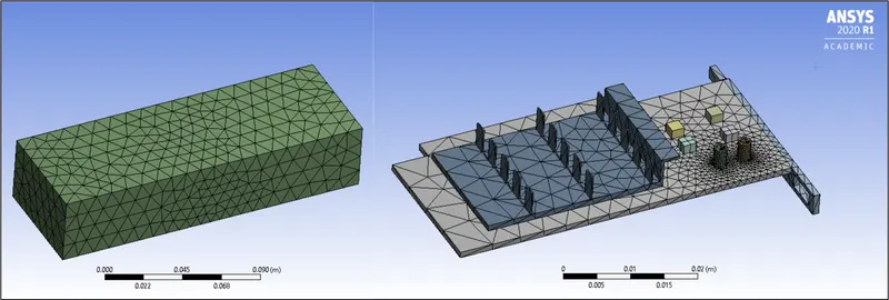
Fig. 2: Baseline Mesh

Mesh	Mesh Element Size [m]	Body Sizing Element Size [m] (Support Bracket)	% decrease in element size (w.r.t Mesh Element Size)	Body Sizing Element Size [m] (Fins Base + PCB)	% decrease in element size w.r.t Body Sizing Element Size (Support Bracket)	Body Sizing Element Size [m] (Processor + Memory Cards)	% decrease in element size w.r.t Body Sizing Element Size (Processor + Memory Card)
Baseline	0.01	0.008	20	0.0064	20	0.00512	20

Table 18: Mesh Element Size and Body Sizing Element Sizes for Baseline mesh of the given graphics card model

Mesh statistics, maximum temperature and wall heat transfer coefficient values obtained by the processor for Baseline Mesh with input velocity of 1m/s:

Mesh	Mesh Element Size [m]	Nodes	Elements	Pressure-Velocity Coupling Scheme	maximum temperature [K]	avg. surface temperature [K]	avg. wall heat transfer coefficient [W m^-2 K^-1] (Eq.1-Eq.4)
Baseline	0.01	13148	68241	SIMPLE	157.503	75.032	43.9545
Baseline	0.01	13148	68241	SIMPLEC	157.432	74.891	43.941
Baseline	0.01	13148	68241	COUPLED	365.276	365.163	43.4877

Table 19: Mesh statistics, maximum temperature, average surface temperature and average wall heat transfer coefficient values obtained by the processor using different Pressure-Velocity coupling schemes for Baseline mesh of the graphics card model with input velocity of 1m/s

Mesh quality attributes for Baseline Mesh:

Mesh	Element Quality(avg.)	Aspect Ratio(avg.)	Skewness(avg.)	Orthogonal Quality(avg.)
Baseline	0.80447	Quadrilaterals+Triangles-2.0549	0.2711	0.72919

Table 20: Mesh quality attributes depicting the average values of element quality, aspect ratio, skewness and orthogonal quality for Baseline mesh of the graphics card model

Section 2.5.2 Mesh Refinement approach

The initial results obtained from the Baseline mesh in Section 2.5.1 Baseline Mesh with regards to the convergence behaviour of the three different algorithms, SIMPLE, SIMPLEC and COUPLED, as can be seen in Fig. 7, Fig. 8, and Fig. 9 and Fig. 10 respectively, it was observed that only the monitor plot with the COUPLED solver demonstrated a highly stable output with both first and second order upwind schemes for the momentum term well before they reach the total number of iterations while the prediction of the same with SIMPLE and SIMPLEC algorithms were oscillating as well as did not show convergence for the energy equation. This implied that only the COUPLED scheme highlighted trends that were closer to the convergence limits based on the residual values mentioned in Table 24 (although the convergence criteria option for all equations were checked off) making the results obtained more reliable and accurate for it to be reused to solve the pressure-velocity equations for the four different meshes that were prepared to obtain a mesh independent solution. It is important to note that the maximum skewness reported for the Baseline Mesh by Fluent was 0.99866, which is more than the recommended value of 0.98 (highly skewed cells lead to convergence difficulties, decreased accuracy and unstable solution), and while results with SIMPLE and SIMPLEC schemes may have varied for a mesh with better skewness, the purpose of the Baseline Mesh was to guide towards an improved mesh refinement strategy that ensured not only the underlying physics was well captured but also the results adhered to the default and a more stricter convergence criteria. The mesh refinement hereafter was created while adhering to the mesh quality attributes mentioned in Section 2.2 Meshing. For the support bracket, fins base and PCB, and Processors, Capacitors and Memory Cards, "Body Sizing" was utilised with percentage decrease between each of the bodies, single and/or combined as shown in Table 21 a), maintained at 20% to minimize errors due to numerical diffusion. "Edge Sizing" was chosen for the surfaces of the PCB Base, Fins Base, Fins, Memory Cards, Capacitors and Processor to uniformly divide the meshing elements and to reduce skewness. The "Edge Sizing" type was selected as "Number of Divisions", as is reported in Table 21 b), and aided significantly in distributing the cell growth evenly around all the surfaces listed before as regions of both coarse and fine mesh existed across the graphics card model.

Mesh	Mesh Element Size [m]	Body Sizing Element Size [m] (Support Bracket)	% decrease in element size (w.r.t Mesh Element Size)	Body Sizing Element Size [m] (Fins Base + PCB)	% decrease in element size w.r.t Body Sizing Element Size (Support Bracket)	Body Sizing Element Size [m] (Processor + Capacitors + Memory Cards)	% decrease in element size w.r.t Body Sizing Element Size (Fins Base + PCB)
1	0.0099	0.00792	20	0.006336	20	0.0050688	20
2	0.009	0.0072	20	0.00576	20	0.004608	20
3	0.0081	0.00648	20	0.005184	20	0.0041472	20
4	0.00729	0.005832	20	0.0046656	20	0.00373248	20

a) Body Sizing Element Size and Mesh Element Size for the four different meshes of the graphics card model

Mesh	Edge Sizing - PCB Base (No. of divisions - In the direction of flow)	Edge Sizing - PCB Base (No. of divisions - In the transverse direction of flow)	Edge Sizing - Fins Base (No. of divisions - In the direction of flow)	Edge Sizing - Fins Base (No. of divisions - In transverse direction of flow)	Edge Sizing - Fins (No. of divisions: Width)	Edge Sizing - Memory Cards (No. of divisions: Length *Width)	Edge Sizing - Processor (No. of divisions: Length *Width)	Edge Sizing - Capacitors (No. of divisions: Along the diameter)
1	32	15	20	5	2	2*2	10*10	9
2	43	20	25	10	4	4*4	12*12	12
3	54	25	30	15	6	6*6	14*14	15
4	65	30	35	20	8	8*8	16*16	18

b) Edge Sizing for the four different meshes of the graphics card model

Table 21: Mesh Element Size, Body Sizing Element Size and Edge Sizing for the four different meshes of the graphics card model

Mesh 1:

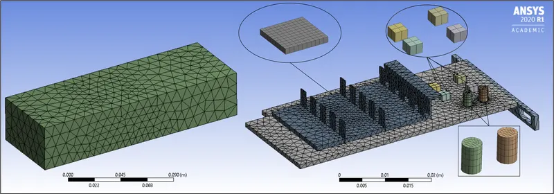
Fig. 3: Mesh 1

Mesh 2:

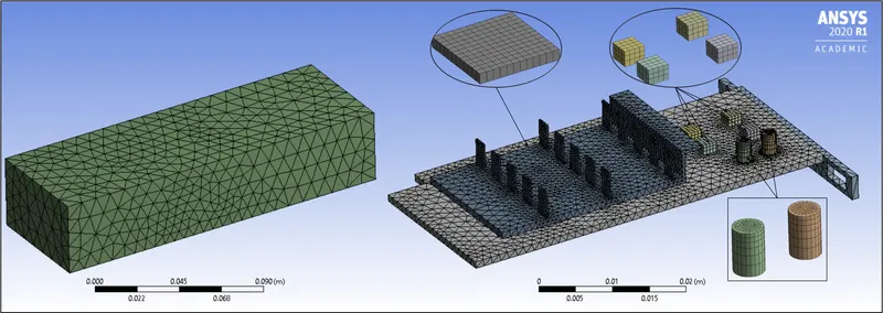
Fig. 4: Mesh 2

Mesh 3:

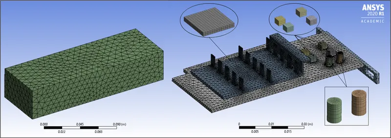
Fig. 5: Mesh 3

Mesh 4:

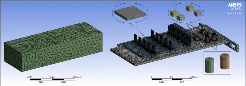
Fig. 6: Mesh 4

Mesh statistics and wall heat transfer coefficient values for the four different meshes:

Mesh	Nodes	Elements	maximum temperature [K]	%var	avg. surface temperature [K]	avg. wall heat transfer coefficient [W m^-2 K^-1] (Eq.1-Eq.4)	%var
1	20080	112622	362.475	--	361.907	43.4975	--
2	41571	234537	361.607	-0.23946	361.03	43.4983	+0.00184
3	64780	364222	360.952	-0.18113	360.339	43.4874	-0.02506
4	90904	508688	360.915	-0.01025	360.299	43.4874	0

Table 22: Mesh statistics, maximum temperature, average surface temperature and average wall heat transfer coefficient values at the processor for different meshes of the graphics card model

Mesh quality attributes for the four different meshes:

Mesh	Element Quality(avg.)	Aspect Ratio(avg.)	Skewness(avg.)	Orthogonal Quality(avg.)
1	0.81485	Triangles and Quadrilaterals - 1.936	0.25757	0.7411
2	0.81915	Triangles and Quadrilaterals - 1.9067	0.25156	0.74722
3	0.82339	Triangles and Quadrilaterals - 1.8918	0.24643	0.75243
4	0.82481	Triangles and Quadrilaterals - 1.8865	0.24399	0.75495

Table 23: Mesh quality attributes depicting the average values of element quality, aspect ratio, skewness and orthogonal quality for the different meshes of the graphics card model

From the meshing statistics in Table 22, mesh number 3 (or mesh 3) with 364222 elements represents a mesh independent result in terms of minimum percentage variation (%var) in the predicted values of maximum temperature and average wall heat transfer coefficient at the processor. The %var is calculated as the ratio of the difference of the predicted values in two consecutive meshes to the predicted value of the previous mesh e.g., ((maximum temperature at the processor for Mesh 2 - maximum temperature at the processor for Mesh 1)/maximum temperature at the processor for Mesh 1). Due to constraints in computational resources and limitations in maximum number of cells/nodes for solution by ANSYS Student license to 512,000 any further reduction in values of Mesh element size, Body Sizing element size and Edge Sizing was not possible to achieve for the given numerical analysis. It should be noted that the value of average wall heat transfer coefficient was evaluated depending on the film temperature for the corresponding solution which implied that the thermal and physical properties of air at that temperature [10] were utilised and as such would result in a more accurate solution owing to its influence surrounding the processor and the graphics card than equivalent values of the same at the inlet. Results in Section 3 will only be referred with regards to the mesh independent solution i.e., Mesh 3.

2.5.3 Convergence Level

As mentioned earlier in Section 2.5.1 Baseline Mesh, three different schemes i.e., SIMPLE, SIMPLEC and COUPLED were compared with regards to convergence study. SIMPLE scheme is iterative in nature, robust (memory efficient) and is quicker per iteration than other pressure-based solvers. SIMPLEC scheme, similar to the SIMPLE scheme, allows increased under relaxation to the pressure correction term that improves in convergence times especially when employed in complicated flows with turbulence and/or supplementary physical models and as such offers greater diversity in terms of computational problems for implementation over SIMPLE scheme. While SIMPLE and SIMPLEC schemes are segregated type of schemes i.e., pressure and velocity terms are updated sequentially, the COUPLED scheme on the other hand updates the pressure and velocity terms simultaneously. This allows the COUPLED scheme to be more efficient in its single-phase implementation especially for steady-state flows offering superior performance over the segregated algorithms (SIMPLE and SIMPLEC) thereby requiring fewer iterations to converge. The selection of schemes for the different terms under spatial discretization included assigning Gradient to Least Squares Cell Based scheme, pressure to second order scheme, momentum to first (for baseline mesh) and second order upwind schemes and energy to second order upwind scheme. Least Squares Cell Based scheme is the default gradient method chosen by ANSYS Fluent which is used to compute the change in values across the centroid of two cells along a vector path and is a computationally less expensive scheme offering comparable accuracy to the node-based gradient scheme, both of which are superior to the cell-based gradient scheme. The second order scheme for the pressure makes use of the central differencing scheme and is generally considered to be more accurate than the Standard and Linear schemes as well as robust in the case of skewed meshes. First order upwind scheme for the momentum term was made use for the baseline mesh, owing to the maximum skewness exceeding the recommended value, which as the name of the scheme suggests is of first order accuracy as it assumes the cell centre values of the field variables to be computed represents cell average values that hold good across a cell as the quantity to be determined at the cell face. A second order upwind scheme is chosen for the momentum (for the refined meshes) and energy terms that makes use of the quantities at the cell face values to compute a cell-centered solution at the cell centroid leading to a second order accurate solution. Convergence criteria option was checked off, however, the residual values which measures the local imbalance of conserved variable in each control volume such as continuity, x-velocity, y-velocity, z-velocity and energy were monitored throughout the solution process for the defined number of iterations, in this case 1000, to allow the actual fluid behaviour to be developed i.e., consistent rate of heat transfer along the shared interfaces between the different solid bodies and the Fluid Volume. The residual limits defined for the laminar viscous model equations and the residual plots corresponding to the different meshes are shown in the table and figures below:

	laminar
continuity	1e-03
x-velocity	1e-03
y-velocity	1e-03
z-velocity	1e-03
energy	1e-06

Table 24: Residual Values of the different equations used in the laminar viscous model

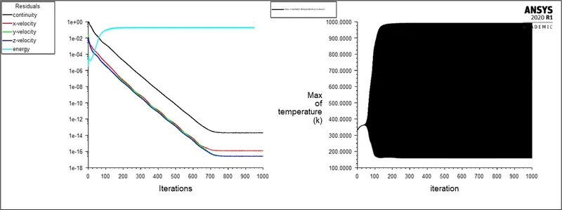
Fig. 7: Scaled Residuals and maximum temperature at processor plots using the laminar viscous model for baseline mesh having input velocity at 1m/s with SIMPLE solver

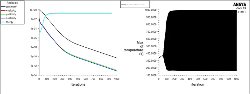
Fig. 8: Scaled Residuals and maximum temperature at processor plots using the laminar viscous model for baseline mesh having input velocity at 1m/s with SIMPLEC solver

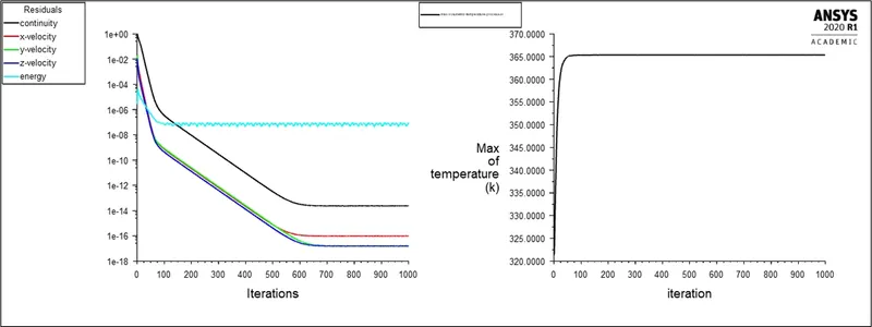
Fig. 9: Scaled Residuals and maximum temperature at processor plots using the laminar viscous model for baseline mesh having input velocity at 1m/s with COUPLED solver (using first order upwind scheme for momentum equation)

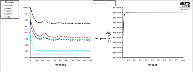
Fig. 10: Scaled Residuals and maximum temperature at processor plots using the laminar viscous model for baseline mesh having input velocity at 1m/s with COUPLED solver (using second order upwind scheme for momentum equation)

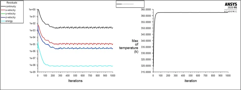
Fig. 11: Scaled Residuals and maximum temperature at processor plots using the laminar viscous model for mesh 1 having input velocity at 1m/s with COUPLED solver

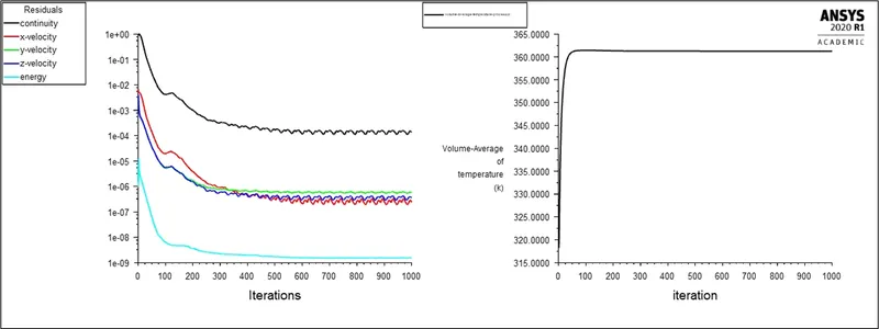
Fig. 12: Scaled Residuals and maximum temperature at processor plots using the laminar viscous model for mesh 2 having input velocity at 1m/s with COUPLED solver

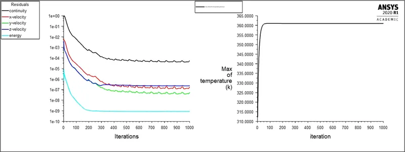
Fig. 13: Scaled Residuals and maximum temperature at processor plots using the laminar viscous model for mesh 3 having input velocity at 1m/s with COUPLED solver

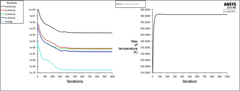
Fig. 14: Scaled Residuals and maximum temperature at processor plots using the laminar viscous model for mesh 4 having input velocity at 1m/s with COUPLED solver

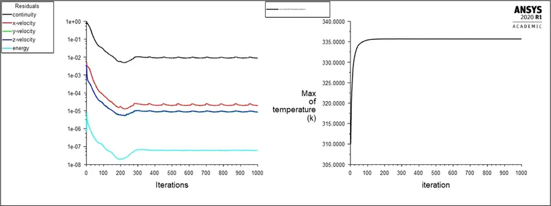
Fig. 15: Scaled Residuals and maximum temperature at processor plots using the laminar viscous model for mesh 3 having input velocity at 2.5m/s with COUPLED solver

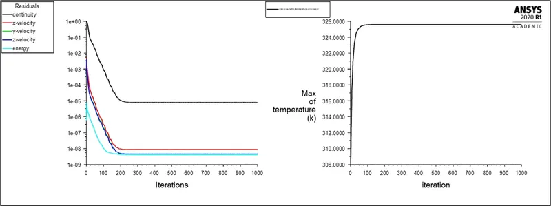
Fig. 16: Scaled Residuals and maximum temperature at processor plots using the laminar viscous model for mesh 3 having input velocity at 5m/s with COUPLED solver

From Fig. 7 and Fig. 8, we can notice that the residuals for SIMPLE and SIMPLEC scheme have not shown stable convergence, as was also reported in Section 2.5.1 Baseline Mesh, and also are converging well above the '1e-06' default limit for energy (although not being considered as the convergence criteria option was checked off) which could be attributed to the Baseline Mesh having maximum skewness greater than the recommended value of 0.98, whereas for the COUPLED scheme (in Fig. 9 and Fig. 10), convergence based on the residual values mentioned in Table 24, except for continuity equation when momentum is set to second order upwind scheme, and maximum temperature monitor plot shows a highly stable output well before they reach the total number of iterations indicating that a steady-state solution has been obtained. This reaffirms the expected behaviour from each of the schemes. Also, using higher order discretization for improved accuracy of the solution which in this case is with momentum being set to the second order upwind scheme, with the exception for mesh1 and mesh3 with input velocity of 2.5m/s wherein continuity equations do not meet the default '1e-03' limit, implying a stricter convergence criteria on the governing equations still yielded stable and converged results as can be seen in the monitor plots from Fig. 11 to Fig. 15. Interestingly, mesh 3 with input velocity of 5m/s did not show convergence with higher order discretization and therefore, momentum was set back to first order upwind scheme with results for residuals and monitor plots as displayed in Fig. 16.

3.Results

In Section 3.1, temperature contour plots (displayed as animation in GIF format), temperature profiles, and velocity vectors along streamwise direction using two different geometry-based definitions i.e., line and plane based, to demonstrate the development of velocity and temperature gradients across the computational domain and especially at the graphics card model at different input velocities with regards to the mesh independent solution are discussed.

3.1 Temperature contour plots, temperature profiles, and velocity vector plots along the flow direction

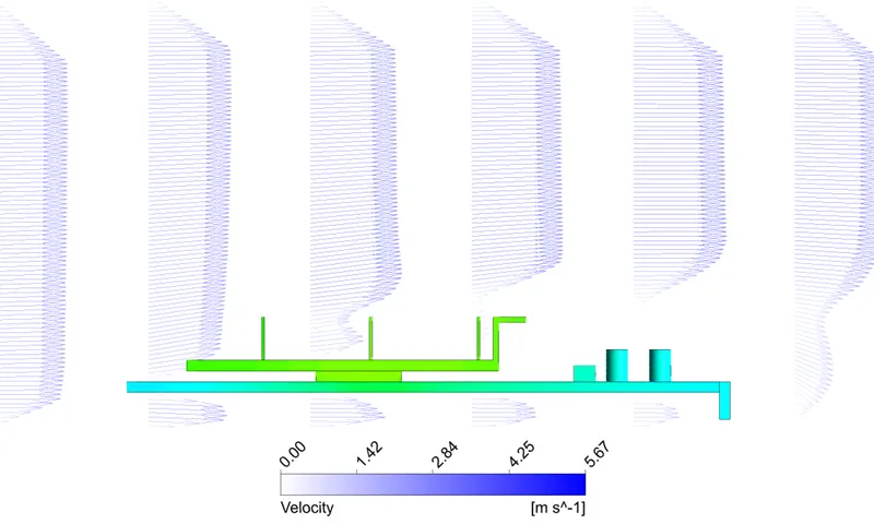
Fig. 17, Fig. 18, Fig. 19, and Fig. 20 shows the velocity and temperature gradients across the computational domain and in the vicinity of the region of the graphics card using temperature contour plots, temperature profiles, and velocity vectors at different line position as tabulated from Table 4 to Table 16 and at Plane 1 in Table 17 respectively. As the flow progresses downstream along the x-axis direction, we notice change in the smoothness of the velocity profile (in Fig. 19) from its pre-existing shape as a result of the incoming geometrical boundaries of the graphics card model. However, both the velocity and temperature profiles (in Fig. 18) are also experiencing effects of the rapidly varying temperature gradient as a result of the dissipated power from the processor of the graphics card. In different regions across the graphics card such as the aluminium fins base, memory cards and capacitor, due to sudden difference in surface areas, a pressure drop is created which causes local velocity in those zones to accelerate as seen in the velocity vector plot in Fig. 20.

For Mesh 3:

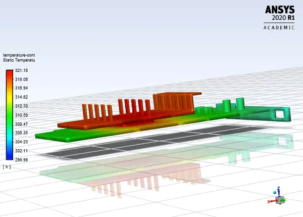
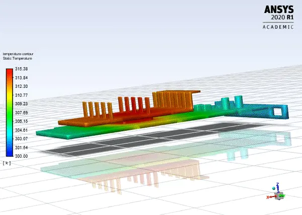
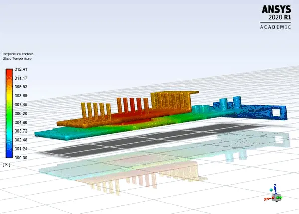
a) Temperature contour at input velocity 1m/s b) Temperature contour at input velocity 2.5m/s c) Temperature contour at input velocity 5m/s

Fig. 17: Temperature contour animation plot for Mesh 3 across the graphics card model for Mesh 3 at different input velocities

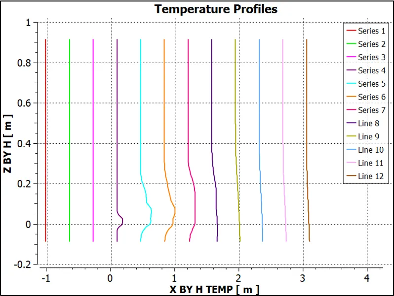
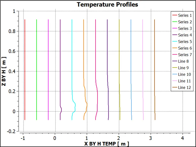
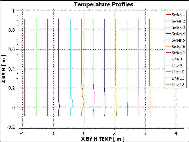
a) Temperature profiles at input velocity 1m/s b) Temperature profiles at input velocity 2.5m/s c) Temperature profiles at input velocity 5m/s

Fig. 18: Temperature Profiles (normalised using model inlet diameter) along x-axis direction for Mesh 3 at different input velocities

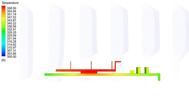
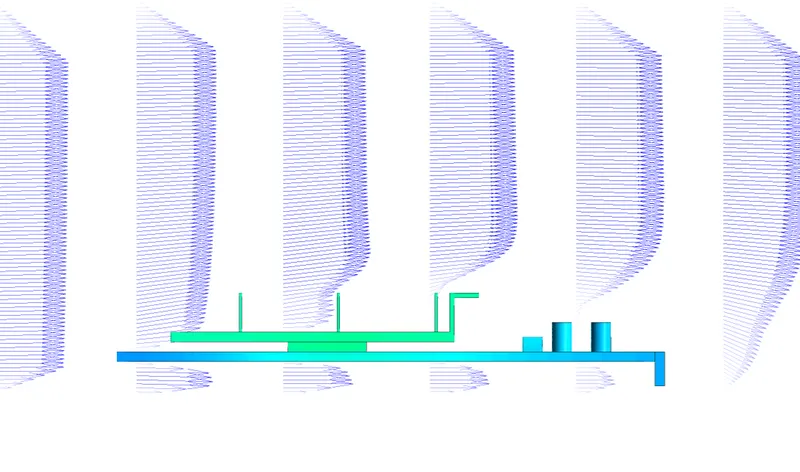
a) Velocity Vectors at input velocity 1m/s b) Velocity Vectors at input velocity 2.5m/s c) Velocity Vectors at input velocity 5m/s

Fig. 19: Velocity Vector plots at different line definitions (as reported from Table 4 to Table 16) for Mesh 3 at different input velocities

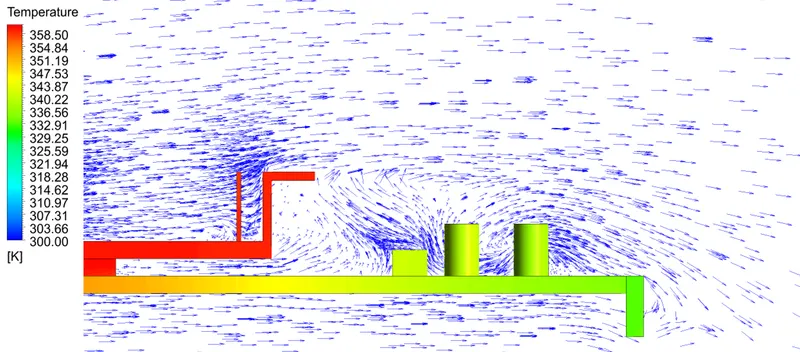
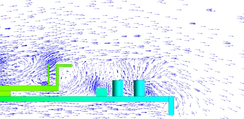
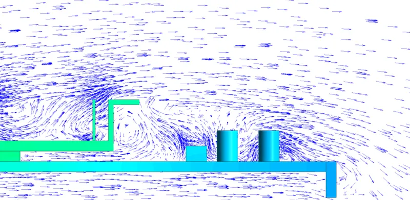
a) Velocity Vectors at input velocity 1m/s b) Velocity Vectors at input velocity 2.5m/s c) Velocity Vectors at input velocity 5m/s

Fig. 20: Velocity Vector Profile within the Fluid Volume domain for Mesh 3 at Plane 3 at different input velocities

Input Velocity [m s^-1]	Reynolds Number (Eq. 1)	maximum temperature [K]	avg. surface temperature [K]	avg. wall heat transfer coefficient [W m^-2 K^-1] (Eq.1-Eq.4)
1	643.087	360.952	360.339	43.4874
2.5	1720.18	335.691	335.098	68.9107
5	3537.74	325.58	324.999	97.5281

Table 25: Reynolds Number, Maximum temperature, average surface temperature and average wall heat transfer coefficient values at the processor for input velocities at 1m/s, 2.5m/s and 5m/s of the given computational model

4. Discussion

Air travelling within the enclosure moves with a parabolic profile with velocity of flow at the walls corresponding to a value of 0m/s due to the "no slip" condition combined with the viscous effects. Since, the governing flow conditions over the graphics card model attributes to the laminar flow regime when compared against an equivalent external flow over flat plate as analogy, the velocity profile remains largely unchanged (also seen in Fig. 19). As the air flow approaches the graphics card model, the velocity profile begins to adjust according to the external features of the geometry, however, due to presence of a sharp temperature gradient across the processor, aluminium fins base and the PCB board, air gets unequally heated in that region adding to further variation in the shape of the profile. The variation of the profile also depends on the incoming velocity from the inlet with the degree of change decreasing for increasing velocity values. Similarly, temperature profiles also vary and are in turn dependent on the flow conditions at the inlet of the enclosed domain. Since, the processor of the graphics card is dissipating a constant TDP value of 150W per unit volume, most of the heat from the source is carried away by the aluminium fins base followed by the PCB board at lower inlet velocity conditions, by mode of conduction due to direct contact, which makes these two zones warmer than the remaining electronic components and as such can be identified as potential hotspots on the model. This condition, however, changes when the incoming air travels at higher values of velocity which makes a significant impact in terms of heat carried away by means of forced convection. It should be noted that the temperature distribution on both the aluminium fins base and the PCB board is highly non-uniform with most of the high temperature areas on both these components concentrated in the region that is shared with the processor surface area. There are a number of flow recirculation regions across the graphics card model, as was mentioned previously due to abrupt change in geometrical features, whose strength varies depending on the gradient to which surface area differs and the governing flow conditions, and as such tends to cause velocity values in that region to arrive at a value of 0m/s thereby hindering the rate of heat transfer by convection. The region beyond the rear end of the aluminium fins base can be located as one of the major flow recirculation regions.

5. Conclusion

The numerical analysis for CHT analysis on a graphics model under steady state conditions for input flow belonging to the laminar regime in ANSYS Fluent 2020 R1 was well understood. The ability of a CFD model to compute the velocity and temperature gradients, especially in the region of the graphics card, with a constant volumetric heat source was realised offering insights into the different modes of heat transfer involved in dissipating the TDP of the processor. Additionally, the average wall heat transfer coefficient computed for the processor walls exposed to the incoming air flow indicated the importance of providing necessary cooling options to reduce thermal damage of the GPU and other electronic components, resulting in improved service life. The presence of large flow recirculation zones identified in this numerical study also strikes importance to the design and improvement of cooling solutions that can further increase rate of heat transfer by convection.

References

[1] Andrew Wheeler 2018, What Raw Materials Are Used to Make Hardware in Computing Devices?, engineering.com, viewed 25 November 2020, <https://www.engineering.com/Hardware/ArticleID/17668/What-Raw-Materials-Are-Used-to-Make-Hardware-in-Computing-Devices.aspx>

[2] Emre Ozturk & Ilker Tari (2007) CFD Modeling of Forced Cooling of Computer Chassis, Engineering Applications of Computational Fluid Mechanics, 1:4, 304-313, DOI:
10.1080/19942060.2007.11015201

[3] Plansee, Tantalum, plansee.com, viewed 25 November 2020, <https://www.plansee.com/en/materials/tantalum.html>

[4] Rebecka Domeij Backryd, Simulation of Heat Transfer on a Gas Sensor Component, Department of Mathematics, Linkopings Universitet, May 2005

[5] Fritz Grensing, Don Hashiguchi, Materion Beryllium & Composites, Data Sheet Mechanical and Thermal Properties of Aluminum-Beryllium AM162, materion.com, viewed 25 November 2020, <https://materion.com/-/media/files/beryllium/albemet-materials/maab-009mechanicalandthermalpropertiesofaluminumberylliumalloyam162.pdf>

[6] Hassan Mujtaba 2016, NVIDIA’s Full Fat Pascal GP104 GPU Pictured With GDDR5X Memory – Features 8 GB Micron Chips To Drive GeForce GTX 1080 Cards, Wccftech.com, viewed 25 November 2020, <https://wccftech.com/nvidia-pascal-gp104-gpu-gddr5x-leak/>

[7] J. R. Culham, M. M. Yovanovich, P. Teertstra, C.-S. Wang, G. Refai-Ahmed, Ra-Min Tain, Sep 2001, "Simplified Analytical Models for Forced Convection Heat Transfer From Cuboids of Arbitrary Shape", Journal of Electronic Packaging, Vol. 123

[8] Yovanovich, M. M., Lee, S., and Gayowsky, T. J., 1992, ‘‘Approximate Analytic Solution for Laminar Forced Convection From an Isothermal Plate,’’ Paper No. 92-0248, AIAA 30th Aerospace Sciences Meeting and Exhibit, Reno, NV, Jan. 6–9.

[9] Lee, S., Yovanovich, M. M., and Jafarpur, K., 1990, ‘‘Effects of Geometry and Orientation on Laminar Natural Convection from Isothermal Bodies,’’ AIAA J. Thermophys., 5, No. 2, pp. 208–216.

[10] Engineers Edge, LLC, Viscosity of air, Dynamic and Kinematic, www.engineersedge.com, viewed 07 December 2020, <https://www.engineersedge.com/physics/viscosity_of_air_dynamic_and_kinematic_14483.htm#:~:text=The%20viscosity%20of%20air%20depends,2%20%2Fs%20or%2014.8%20cSt.>