Week 12 - Validation studies of Symmetry BC vs Wedge BC in OpenFOAM vs Analytical H.P equation

1. Introduction

In this challenge, similar to the previous one (Week 11), the aim was to perform a two-dimensional transient axi-symmetric numerical simulation of an incompressible-laminar-viscous flow across a pipe of constant cross-section with flow characteristics resembling inlet conditions at Reynold's number of 2100, however, using the wedge and symmetry boundary conditions for different angles with the center viz., 10°, 25° and 45°. The MATLAB script demonstrating the automation capabilities with regards to generation of the blockMeshDict file was reused from the previous challenge and the corresponding results obtained from the numerical simulation were validated against the Hagen-Poiseuille's equations for the fully developed flow condition.

2. Method

The typical approach adopted to performing numerical simulation in OpenFOAM involves the following steps:

1. Identifying the tutorial in the 'FOAM_TUTORIALS' folder that contains the appropriate governing equations relevant to the physics of the flow for the given problem. A typical file structure of an OpenFOAM tutorial consists of the below mentioned directories and files:
1. A 'system' directory with the 'controlDict', 'fvSchemes' and 'fvSolution' files used for specifying the numerical schemes and solution procedure along with control on the simulation run properties. Additionally, for the given numerical problem, a file by the name 'blockMeshDict' mentions the creation of a hex block representing the geometry as well as its mesh properties.
2. A 'constant' directory that contains a 'polyMesh' directory outlining the various aspects of the mesh such as 'boundary', 'points', 'faces', etc., and a file that defines the physical properties, in this case, 'transportProperties' specifying the value of kinematic viscosity.
3. A time directory, usually called the '0' directory that consists of files representing the different fields or fluid flow properties with values as required at the start of simulation run or at time `t = 0`.
2. Copying the now identified tutorial folder from the 'FOAM_TUTORIALS' folder to the 'FOAM_RUN' folder, specifically created to allow simulation run of OpenFOAM numerical simulation cases, with either the same name or preferably a name relevant to the geometry to be discretized.
3. Replacing the geometry and boundary list of the pre-existing tutorial with the geometry and boundary list pertaining to the given problem and defining mesh parameters with regards to the flow physics, in this case by updating the 'blockMeshDict' file (Section 2.1 Modelling).
4. Updating the 'transportProperties' file with kinematic viscosity value of water at 25°C (Section 2.2 Evaluation of inlet velocity from Reynolds number and entrance length).
5. Updating the fields' files present inside the '0' directory viz., 'U' and 'p', with the boundary list as specified in the 'blockMeshDict' file and appropriate values at the relevant boundary to ensure the given numerical problem has the right boundary conditions and that the solution would be correctly initialised (Section 2.3 Boundary Conditions).
6. Updating the 'controlDict' file, in this case the 'deltaT' and 'endTime' parameters with values that take into consideration domain specific attributes such as length of the pipe in the direction of flow, fluid flow velocity and avoiding violation of Courant-Friedrichs-Lewy Condition or the CFL number by limiting its mean and maximum value during simulation run below 1 (Section 2.5 Determination of transient parameters).

The above steps were executed using Linux commands in a Ubuntu 20.04.2.0 LTS (Long Term Support) operating system as shown below:

i) Change directory to FOAM_RUN:

cd $FOAM_RUN

ii) Copy cavity example from FOAM_TUTORIALS directory that contains the icoFoam solver to the FOAM_RUN directory:

cp -r $FOAM_TUTORIALS/incompressible/icoFoam/cavity/cavity .

iii) Rename cavity directory to Week_12_flow_through_pipe_simulation

mv cavity Week_12_flow_through_pipe_simulation

iv) Change directory to Week_12_flow_through_pipe_simulation

cd Week_12_flow_through_pipe_simulation

v) Replacing the geometry and boundary list by editing the 'blockMeshDict' file:

gedit system/blockMeshDict

vi) Updating the kinematic viscosity value by editing the 'transportProperties' file:

gedit constant/transportProperties

vii) Updating the boundary list and boundary conditions by editing the 'U' and 'p' files:

gedit 0/U

gedit 0/p

viii) Updating the 'deltaT' and 'endTime' parameters with appropriate values by editing the 'controlDict' file:

gedit system/controlDict

ix) Creating the block based geometry and generating mesh for the computational domain:

blockMesh

x) Running the icoFoam solver to solve for the incompressible laminar Navier-Stokes equations:

icoFoam

xi) Post-processing and visualising results of the performed simulation (Section 2.5):

paraFoam

The names of the directory starting with 'Week_12_flow_through_pipe_simulation' were further extended by the addition of '_wedge_angle_' with the text appearing at the end of '_' in 'wedge_angle_' representing the value of the wedge angle for which the numerical simulation was to be performed and similarly, after the value of the wedge angle, the boundary condition 'symmetry' or 'wedge' was attached. For example, the directory for 'Week_12_flow_through_pipe_simulation' with wedge angle as 25° using the symmetry boundary conditions would read as follows:

'Week_12_flow_through_pipe_simulation_wedge_angle_25_symmetry'

2.1 Modelling

The problem was modelled using the same single three-dimensional hexahedral block (number of mesh elements in y-direction was set to 1 for a two-dimensional axi-symmetric flow problem) from the previous challenge resembling a cut-section of the pipe, similar to an elongated wedge (as seen in Fig. 1), whose angle with the centre varied between 10°, 25° and 45°, with the block defined using 6 vertices by collapsing its bottom face or in other words, merging vertices on the bottom side of the front and back faces that were adjacent to the bottom face, in a dictionary type file called 'blockMeshDict'. The total number of grid points reflected the mesh independent setup from the previous challenge wherein the number of cells along z-axis and x-axis directions was 1200 and 69 respectively. The meshing approach adopted for the given computational domain was developed to maintain the meshing quality attributes viz., aspect ratio, skewness and non-orthogonality, within the ranges outlined by CFD support [1] in the following table:

Aspect Ratio	1 - Best possible value
Skewness			<20 although higher values affect the accuracy of results
Orthogonal Quality	n0<70 (Safe Values)	70<n0<90 (requires special treatment)	n0>90 (unacceptable)

Table 1: Mesh Quality Attributes as defined by CFD support [1]

The reason for targeting the above mentioned mesh quality attributes comes from analysis across different types of flow problems that these are few of the known ways of identifying whether the discretized mesh would develop convergence issues during the solution process and to avoid fatal solver scenarios.

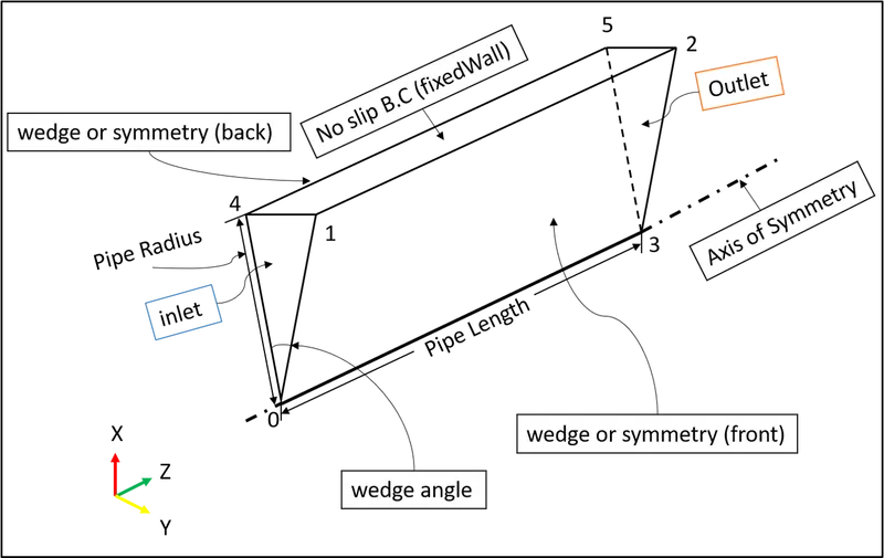
Fig. 1: Pipe flow Geometry (single hexahedral block and vertices representing the decomposed main domain, and boundary conditions)

Mesh for Wedge angle of 10°:

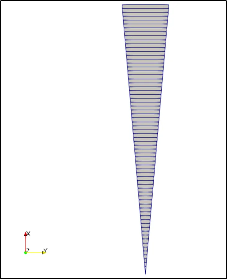
Fig. 2: Mesh for Wedge angle of 10° (View from inlet)

Mesh for Wedge angle of 25°:

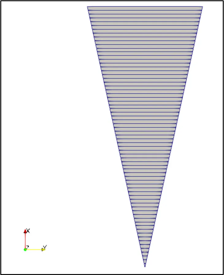
Fig. 3: Mesh for Wedge angle of 25° (View from inlet)

Mesh for Wedge angle of 45°:

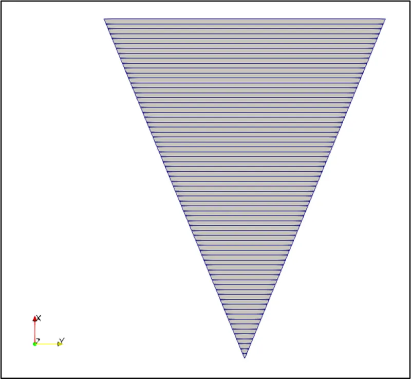
Fig. 4: Mesh for Wedge angle of 45° (View from inlet)

Mesh statistics and quality attributes for the different meshes:

Wedge Angle (°)	Constraint Type	Cells	Max Aspect Ratio	Max Skewness	Max Non-Orthogonality
4	Wedge	82800	27.6166	0.331709	0
10	Wedge	82800	27.7053	0.323205	0
10	Symmetry	82800	158.337	0.331709	0
25	Wedge	82800	28.27	0.554025	0
25	Symmetry	82800	63.759	0.554025	0
45	Wedge	82800	29.874	1.0354	0
45	Symmetry	82800	57.1609	1.0354	0

Table 2: Mesh statistics and quality attributes depicting the maximum values of aspect ratio, skewness and non-orthogonality for different wedge angles and constraint types

Mesh quality attributes of all the different meshes prepared in Table 2 indicates that while the maximum aspect ratio increases with increase in the wedge angle for the wedge boundary condition, a decrease in the same was noticed with increase in the wedge angle for the symmetry boundary condition despite the geometry aspects of the meshed domain for the same wedge angle using the 'checkMesh' command such as 'Overall domain bounding box', 'minimum face area', 'maximum face area', and 'Total volume' reporting the same and a possible reason could not be determined. The maximum skewness determined also demonstrated increase in its value with increase in the wedge angle as the distance increases for the resulting intersection formed by the line connecting two cell centres with their common face and the centre of that face. However, maximum non-orthogonality values remain unaltered as the angle formed between the line joining two cell centres and the normal of the face common to them remained the same due to the number and quality of cells across the domain continuing to retain at a total of 82800 and of the type hexahedra and prisms respectively with the number of cells in the case of the former type (hexahedra) as 81600 while the latter type (prisms) at 1200 being constant.

2.2 Evaluation of inlet velocity from Reynolds number and entrance length

Reynolds number, based on the inlet pipe diameter, can be expressed below as:

`Re = (U*L)/nu`, where (Eq. 1)

`U` is the inlet velocity,

`L` is the characteristic length, in this case, the inlet diameter of the pipe, and

`nu` is the kinematic viscosity of fluid i.e., water at 25°C

Substituting the value of given Reynolds number as 2100, inlet diameter of pipe selected as 0.01m and kinematic viscosity of water at 25°C as 8.9e-7 [2] in (Eq. 1), we get inlet velocity of water flowing through the pipe as 0.1869m/s.

The entrance length, as seen in the previous challenge, for laminar flow, in non-dimensional form, can be expressed mathematically as shown below:

`(L_h)/D cong 0.05*Re` (Eq. 2)

Substituting the values of inlet diameter of pipe and Reynolds number in (Eq. 2), the entrance length or Hydro-dynamic length was evaluated to a value of 1.05m from the inlet of the pipe geometry in the direction of flow.

2.3 Boundary Conditions

The different regions of the mesh, identified as patches, that demarcate its extents as well as specify the boundary conditions to be employed on them is written in a list called as 'boundary' in the 'blockMeshDict' file. The input and output data in OpenFOAM are recorded as tensor fields which are written onto time directories, in this case the fields being velocity ('U') and pressure ('p') in the '0' folder, and read from it at an appropriate time. A typical structure of the field data file consists of the 'dimensions' written with 7 scalars representing the 'dimensionSet' enclosed by square brackets with each scalar highlighting the properties of mass, length, time, temperature, quantity, current and luminous intensity respectively from left to right in base units for SI and USCS, 'internalField', in this case of type 'uniform', that allocates a single value to all elements within the field and expressed using 3 vector components for velocity (U) and only 'uniform 0' for pressure (p) as it is kinematic pressure for an incompressible case for which its absolute value is of little significance, and 'boundaryField' which consists of a list of boundary conditions and data for all patches, preferably identical in name to the patches created in 'boundary' in the 'blockMeshDict' file. For the given numerical simulation, the different patch names and patch types of the 'blockMeshDict' file and boundary fields (type and value) of the time directory files, 'U' and 'p', describing the numerical simulation of an incompressible-laminar-viscous flow through the pipe geometry are similar to the previous challenge except for the introduction of type 'symmetry' in place of the type 'wedge' boundary condition and is mentioned in the following table:

patch name	inlet	outlet	fixedWall	front	back	axis
patch type (in blockMeshDict)	patch	patch	wall	wedge/symmetry	wedge/symmetry	empty
type (in U)	fixedValue	zeroGradient	noSlip	wedge/symmetry	wedge/symmetry	empty
value (in U)	uniform(0 0 0.1869)	--	--	--	--	--
type (in p)	zeroGradient	fixedValue	zeroGradient	wedge/symmetry	wedge/symmetry	empty
value (in p)	--	uniform 0	--	--	--	--

Table 3: Boundary Conditions and its setup

Type 'zeroGradient' in '0' time directory files, 'U' and 'p', indicates the normal gradient of that particular field at the relevant patch name is 0, type 'noSlip' is used to set the velocity of the 'fixedWall' patch to (0 0 0), type 'empty' for the 'axis' patch is used in two dimensional flow problems indicating that the plane on this surface is normal to the third dimension which requires no solution, type 'wedge' is used in two-dimensional axi-symmetric cases, in this case the pipe representing a cylinder is specified as a wedge of certain angle with the center that is 1 cell (or element) thick extending across the centerline while type 'symmetry' defines 'slip' condition on a non-planar patch.

2.4 icoFoam model

The icoFoam solver uses the PISO pressure-velocity coupling algorithm to solve the incompressible laminar Navier-Stokes equations. The Navier-Stokes equations define the fluid flow properties such as velocity, pressure, density, temperature, viscosity, energy, etc., within a given physical domain. Additionally, the Navier-Stokes equations are developed with regards to the laws of conservation that states the net mass flow across a system is zero (Conservation of mass), momentum within the same system (or control volume) is constant (Conservation of momentum). The continuity and momentum equations are mathematically expressed below as:

Continuity equation: `nabla*U = 0`

Momentum equation: `del/(del t)*(u) + nabla*(uotimesu) - nabla*(nu*nablau) = -nabla p` ; where

`u` is velocity (in m/s), and

`p` is kinematic pressure (in `m^2/s^2`)

2.5 Determination of transient parameters

The setup of simulation run time and time-step size for any given computational domain in OpenFOAM is described in the 'controlDict' dictionary file. Typically, the start of any simulation begins at `t = 0`, in which case OpenFOAM is required to read the field values of the '0' directory and therefore 'startFrom' keyword is set to 'startTime' which is in turn set to 0 referring to the '0' directory. The 'endTime' depends on the domain length and the flow velocity, in the direction of flow, such that the fluid medium passes through it at least 10 times to acquire steady state conditions, in the case of laminar flow as a mark of a general rule and also as a recommendation in the OpenFOAM v8 User Guide. The steps shown below are identical to that of the previous challenge and therefore, 'endTime' was evaluated as:

`endTime = (L/U)*10`; where (Eq. 3)

`L` is the length of the computational domain = 1.2m, and

`U` is the fluid flow velocity = 0.1869m/s

Since, the length of the domain remains unchanged from the previous challenge, we get the same value of 'endTime' from Eq. 3 to be approximately as 64.205s rounded to the nearest whole number at 65s. Time-step size, 'deltaT' was decided based on the CFL number which is expressed below:

`CFL = (U*Delta t)/(Delta z)`; where (Eq. 4)

`Delta t` is time-step size,

`Delta z` represents the smallest cell size, which was calculated as the ratio of length of the computational domain to the number of mesh elements in the direction of flow, in this case along z-axis direction, i.e.,

`Delta z = L/n_z`; (Eq. 5)

In order to attain temporal accuracy and numerical stability using the 'icoFoam' solver, the CFL criteria was required to be less than 1 and therefore, the value of time-step size was initially determined with the limiting value of the CFL criteria as 1 and tabulated as shown below:

`Delta z` (in m) (Eq. 5)	Time-step size (`Delta t`) (in s) (Eq. 4)
0.001	0.00535

Table 4: Smallest element size (`Delta z`) and time-step size (`Delta t`) values

The above calculated value of time-step size in Table 4 resulted in the mean Courant number to report values less than 1, however, the maximum Courant number continued to be greater than 1. Therefore, the time-step size was further reduced to 0.0025s for wedge angles of 10° and 25°, and 0.0024s for wedge angle of 45° respectively as a trade-off between computational time and the maximum Courant number reporting values just under 1.

2.6 Post-Processing

The steps for post-processing remain the same from the previous challenge, wherein the velocity profiles were plotted at the Hydro-dynamic length from the inlet of the pipe geometry by using ParaView's in-built "plot over line" tool. The "plot over line" tool was accessed by clicking on 'Filters' present in the data analysis group, followed by entering the coordinates as seen in Table 5, and then clicking on the "Apply" button to view the said profile. Similarly, the pressure profile across the entire domain was represented using the "plot over line" tool, however, with coordinates as depicted in Table 6. Visualisation of the wall shear stress plot was essentially a four-step process which has been described briefly as follows:

1. Determination of the magnitude of velocity (U) using the calculator tool:
1. Select the calculator tool from the common toolbar which needs to be enabled, usually selected by default, by accessing the same in the 'Toolbars' option of the 'View' menu.
2. Enter an appropriate 'Result Array Name' such as 'mag_U' in the 'Properties' tab of the calculator tool window and select 'mag' (as in Magnitude) item from the 'Scalars' drop-down option in the calculation box followed by round open and close brackets and then 'U' (for Velocity) item from the 'Vectors' drop-down option such that the text reads 'mag(U)' before clicking on the 'Apply' button.
2. Evaluate the gradients for magnitude of velocity (U) using the 'Gradients of unstructured data set' tool:
1. Select the 'Gradients of unstructured data set' tool by either typing the same in the search window enabled by pressing 'Ctrl+Space' on the keyboard or through the search option from the 'Filters' menu.
2. Type an appropriate 'Result Array Name' such as 'grad_mag_U' in the 'Properties' tab of the 'Gradients of unstructured data set' tool window and select 'mag_U' created in point b. of step i., 'Determination of the magnitude of velocity (U) using the calculator tool', as the 'Scalar Array' before clicking on the 'Apply' button after which the 'grad_mag_U' quantity would appear inside the Field Variable selection box.
3. Computing the wall shear stress variable:
1. Repeat all the steps in point i., 'Determination of the magnitude of velocity (U) using the calculator tool', however ensuring that the 'Result Array Name' is typed as tau (representing wall shear stress) and the calculation box appears as 'grad_mag_U*0.00089' which was entered by selecting 'grad_mag_U' from the 'Vectors' drop-down option followed by multiplying it with the value 0.00089 which is the dynamic viscosity of water at 25°C (expressed in kg/ms) before clicking on the 'Apply' button after which this quantity like the 'grad_mag_U' quantity from point ii., 'Evaluate the gradients for magnitude of velocity (U) using the 'Gradients of unstructured data set' tool', would appear inside the Field Variable selection box.
4. Plotting wall shear stress:
1. Using the "plot over line" tool as mentioned previously in this section, wall shear stress was plotted at the same coordinates as that of the velocity profile in Table 5.

It was ensured that the last time-step size of the simulation run was selected to view the pressure results, and velocity and wall shear stress profiles. In order to compare numerical simulation results of velocity and wall shear stress profiles for different wedge angles and constraint types against their analytical counterparts for validation, following expressions were created, one at a time, in the calculation box of the calculator tool with the term on the left-hand side of both the equations as the 'Result Array Name' in the 'Properties' tab of the same tool before plotting them at the coordinates as seen in Table 5:

Expressions:

Analytical Velocity Profile:

U(r)_analytical = 2*0.1869*(1-((coordsX)^2/(0.005^2)))

Analytical Wall Shear Stress Profile:

tau_analytical = 0.00089*2*0.1869*(1-((2*coordsX)/(0.005^2)))

Legends, titles, and x and y labels were added for better understanding of the graphical representations.

Line	x	y	z
Point 1	0	0	1.05
Point 2	0.005	0	1.05

Table 5: Line Coordinates for viewing the velocity and wall shear stress profiles

Line	x	y	z
Point 1	0.0025	0	0
Point 2	0.0025	0	1.2

Table 6: Line Coordinates for viewing the pressure profile

3. Results

3.1 Validating the Hydro-dynamic length and fully developed flow velocity profile with the numerical results

Fig.5 below shows the fully developed flow velocity profiles for both the analytical and numerical simulation results for different wedge angles and constraint types at the Hydro-dynamic length of 1.05m from inlet of the pipe geometry. It can be observed that the velocity profiles obtained from the numerical simulation results shows better agreement with increasing wedge angle against the analytical velocity profile towards the peak region, however, for the remaining sections of the curve length, the deviations become more profound. The curves representing the velocity profile for the same wedge angle but different constraint types viz., type 'wedge' and type 'symmetry' boundary conditions have almost similar values and are therefore overlapping making it difficult to distinguish them from each other along the arc length.

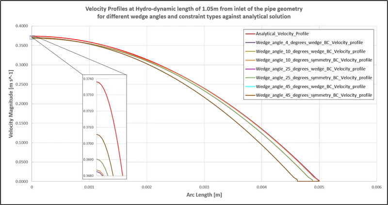
Fig. 5: Velocity profile plots at Hydro-dynamic length of 1.05m from inlet of the pipe geometry for different wedge angles and constraint types against analytical solution

3.2 Validating the maximum velocity and pressure drop for fully developed flow with the numerical results

Maximum velocity, in the case of fully developed flow laminar flow, is derived from the analytical velocity profile specified in Section 2.6 Post-Processing under Expressions leading to the inference that average velocity is equivalent to one half of the maximum velocity. The expressions for analytical velocity profile and the resulting maximum velocity [3] have been mathematically expressed below as:

Analytical Velocity Profile:

`u(r) = 2*V_(avg)*(1-(r^2)/(R^2))`; where (Eq. 6)

`V_(avg)` is the average velocity, in this case the fluid flow or input velocity `U`,

`R` is the radius of the pipe, and

`r` is the position/coordinate location along the radius of the pipe

Maximum velocity is obtained by substituting `r` as 0 representing centerline position in (Eq. 6):

`u_(max) = 2*V_(avg)` (Eq. 7)

Substituting the values of input velocity in (Eq. 7), we get maximum velocity for analytical solution as 0.3738m/s.

Pressure drop, on the other hand, is demonstrated by the difference in the pressure values across the domain, in this case the pipe geometry, and can be expressed mathematically with regards to the Hagen- Poiseuille's equations for the fully developed flow as shown below:

`Delta P = (32*mu*L*V_(avg))/(D^2)`; (Eq. 8)

It should be noted that the pressure drop expressed in (Eq. 8) has S.I units of the form [kg m s^-2] while pressure values recorded by OpenFOAM with the icoFoam solver has S.I units of the form [m^2 s^-2] representing kinematic pressure as was also mentioned in Section 2.3 Boundary Conditions and Section 2.4 icoFoam model. Therefore, to compare the computed pressure drop from numerical simulation against the analytical solution, pressure drop was determined by first substituting the values of the length of the domain (in m), dynamic viscosity of water at 25°C (expressed in kg/ms), input velocity (in m/s) and inlet diameter of the pipe in (Eq. 8) followed by dividing by the density of water at 25°C equivalent to 997 (kg/m^3) which yielded a value of 0.06407 (m^2/s^2).

From the maximum velocity values, as seen in Table 7, it can be seen that the deviations reduced from 1.484% for wedge angle of 4° to almost 0.868% for wedge angle of 45° when compared against the analytical solution and therefore the values tend to arrive at closer confirmation with each other. However, the pressure drop computed by the numerical simulation increases from 32.644% for wedge angle of 4° to more than 50% for wedge angle of 45° against the analytical solution for the same in Table 7 and this may be a result of the aggregated losses in accuracy of values of the constants used for evaluation of the term concerned and/or the lack of a finer grid spacing in the direction of flow, which due to constraints on computational resources was considered as a suitable trade-off. Similar to the velocity profiles, the curves representing the pressure profiles in Fig. 6 for the same wedge angle but different constraint types viz., type 'wedge' and type 'symmetry' boundary conditions have almost similar values and are therefore overlapping making it difficult to distinguish them from each other along the arc length.

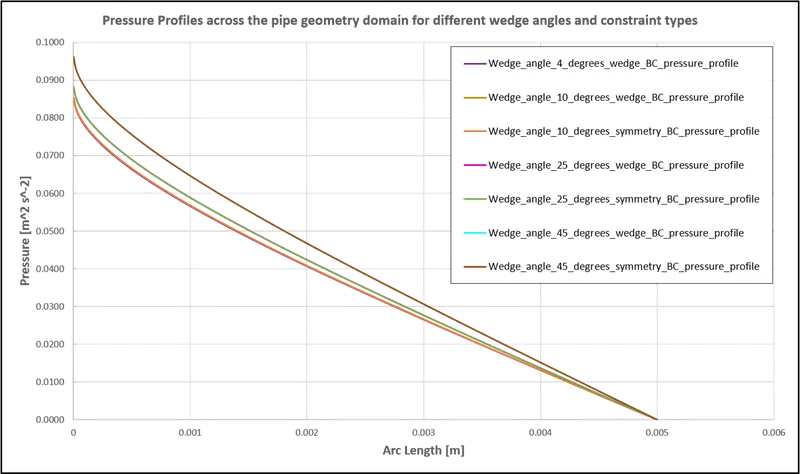
Fig. 6: Pressure profile plots across the pipe geometry domain for different wedge angles and constraint types against analytical solution

Geometry, time statistics, maximum velocity and pressure drop values for different wedge angles and constraint types:

Wedge Angle (°)	Constraint Type	Execution Time [s]	Clock Time [s]	Maximum Velocity [m s^-1]	% var against maximum velocity for Analytical Result	Pressure Drop [m^2 s^-2]	% var against pressure drop for Analytical Result
4	Wedge	10162.2	10169	0.368253	1.484	0.084985	32.644
10	Wedge	10016.8	10022	0.368366	1.454	0.085409	33.306
10	Symmetry	12615.4	12617	0.368367	1.453	0.085409	33.306
25	Wedge	9787.28	9789	0.369036	1.274	0.0881328	37.557
25	Symmetry	12190.8	12192	0.369036	1.274	0.0881328	37.557
45	Wedge	10993.7	10996	0.370557	0.8676	0.0961455	50.063
45	Symmetry	13014.8	13024	0.370556	0.8678	0.0961455	50.063

Table 7: Geometry, time statistics, maximum velocity and pressure drop values for different wedge angles and constraint types and their % var against analytical solutions (Eq. 7 and Eq. 8)

3.3 Validating the wall shear stress for fully developed flow with the numerical results

In Fig.7 below, we can notice the wall shear stress profiles, similar to the velocity profiles, depart away from the analytical profile for the same with increasing wedge angles at the Hydro-dynamic length of 1.05m from inlet of the pipe geometry based on fully developed flow conditions. Again, just like the velocity profiles in Fig. 5 and pressure profiles in Fig. 6, the curves representing the wall shear stress profiles for the same wedge angle but different constraint types viz., type 'wedge' and type 'symmetry' boundary conditions have almost similar values and are therefore overlapping making it difficult to distinguish them from each other along the arc length.

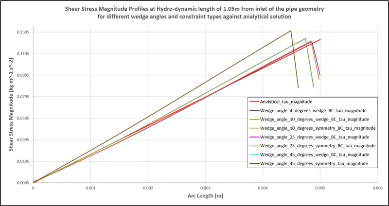
Fig. 7: Wall Shear Stress magnitude profile plots at Hydro-dynamic length of 1.05m from inlet of the pipe geometry for different wedge angles and constraint types against analytical solution

4. Discussion

The fluid flowing across the pipe undergoes transformation in its profile from a uniform shape at the entrance to a parabolic shape downstream due to increasing presence of the viscous effects causing the development of a boundary layer as a result of its movement along the wall of the pipe offering the "no slip" condition leading the velocity of flow at the wall surface to arrive at a value of 0. At the fully developed flow condition, the velocity profile and wall shear stress represented by the slope of the velocity profile at the wall surface remains unaltered. A similar trend is also observed from the numerical simulations performed, however, as the wedge angle increases, the shape of the parabolic velocity profile and wall shear stress plots deviates from their analytical solutions due to change in the size of the cell structure attempting to fit the boundary although they continue to remain of the type hexahedra and prisms. Similarly, the pressure drop plot reports higher values with increasing wedge angles and this too can be attributed to the variation in the size of the cell impacting the values computed across the faces and at the center of the cell. The difference between the wedge constraint type for wedge angle of 4° and symmetry boundary condition for remaining wedge angles of 10°, 25° and 45° can be reasoned on the grounds that the wedge constraint type is a unique case of cyclic boundary condition that takes into consideration only a single cell pertaining to each wedge-face-pair allowing for rotational flow around the axis which also makes the results from the former (wedge boundary condition for wedge angle of 4°) have better correlation with regards to the analytical profiles of velocity and wall shear stress as a closer approximation is obtained compared to the latter. The effect of wedge constraint type on wedge angles of 10°, 25° and 45° shows negligible difference with the symmetry constraint type for the same angles which makes the wedge constraint type ineffective and is therefore recommended to be applicable for angles less 5°.

5. Conclusion

The numerical simulation of flow through a cut section of the pipe geometry using the wedge and symmetry boundary condition for wedge angles of 10°, 25° and 45° in OpenFOAM was well understood. It was realised that while the maximum velocity computed using symmetry boundary condition showed better correlation with increasing wedge angles, wedge constraint type for wedge angle of 4° demonstrated the closest prediction when compared to the analytical profiles of velocity and wall shear stress as well the least variation against analytical pressure drop values for the same mesh configuration. Additionally, the wedge boundary condition is most effective when the wedge angle is less than 5° and the difference against the symmetry constraint type at higher wedge angles becomes less pronounced.

6. References

[1] CFD Support, Mesh Quality Check, www.cfdsupport.com, viewed 17 March 2021, <https://www.cfdsupport.com/OpenFOAM-Training-by-CFD-Support/node131.html>

[2] The Engineers Toolbox, Water - Dynamic and Kinematic Viscosity, www.engineeringtoolbox.com, viewed 16 March 2021, <https://www.engineeringtoolbox.com/water-dynamic-kinematic-viscosity-d_596.html>

[3] Yunus A. Cengel & John M. Cimbala, 2018, Fluid Mechanics: Fundamental and Applications, Fourth Edition, McGraw-Hill Education