Gearbox Sloshing effect

1. Introduction

Gearboxes, over the years, have served the purpose of using a system of gears to alter torque and speed in various forms and in a variety of different meshing configurations between them including in industrial machinery, conveyors and aerospace to name a few examples from the huge list of rotary motion power transmission applications and industries. Since, the gears involved are in physical contact with each other to perform the required operation, after a certain period of time and depending on the environmental conditions to which they are exposed, wear and tear would occur between them leading to eventual failure. Therefore, in order to reduce or carry away the heat generated during rolling or sliding friction as well as to limit the rising temperature as a consequence for improved service life, it becomes paramount to lubricate the gears. Gearbox lubrication can be classified into three methods viz., grease lubrication, splash lubrication and forced oil circulation lubrication and the use of each of them particularly depends on the tangential and rotating speed. Splash lubrication works best with helical, spur and bevel gearboxes at medium and/or high speeds wherein the gears are immersed in oil, typically partially, and is therefore also referred to as oil bath. The rotational motion of gears using the splash lubrication method carries the oil along the surface of individual gear teeth and between adjacent gear teeth on the same gear which then gets splashed onto teeth of other gear(s).

The aim of this challenge is to perform transient simulations using different fluid and lubricating oil combinations, the fluid being air, for a gearbox undergoing splash lubrication at different immersion values for the gears. The motion of the gears within the gearbox are pre-determined with the help of a user-defined function (UDF). A UDF in ANSYS Fluent can be described as a C or `C^(++)` function, dynamically loaded, that offers enhanced standard features and finds uses in solution initialisation, customized boundary conditions, defining material properties, surface and volume reaction rates as well as source terms mentioned by both Fluent and user-defined scalar (UDS) transport equations to list a few [1]. During the gear motion, the lubricant carried across the different parts of the gearbox may undergo severe variations in its transport profile, typically caused as a result of external forces acting on the housing, leading to a rather violent and resonant fluid motion or wave motions described as sloshing effect. Since, the lubricant is contained within the gearbox, the fluid-structure interaction with regards to the constantly changing pressure values, as a result of the sloshing effect, can lead to structural damage and an electrostatically charged mist that can be dangerous. This numerical analysis involves study on two different meshes, one finer or more refined than the other, and as the shape of the domain consisting of the fluid-lubricant mixture was changing as a function of time due to the employed motion on the gears by a UDF, a dynamic mesh model was used to allow this movement to be captured more accurately by adjusting the mesh corresponding to the flow and were defined with respect to the quality attributes of the two meshes mentioned previously with which results are computed for the volume fraction representation of the fluid-lubricant mixture. Dynamic meshing has also found great importance in applications such as simulation of flap movement of an airplane wing for improved resolution and representation on velocity and pressure profiles, combustion of solid fuels and determining the height during burning of fuel, tidal turbine analysis and modelling of an underwater vehicle in submerged and non-submerged situations.

2. Method

2.1 Modelling

The computational domain for simulating flow of fluid and lubricating oil combination around the gears of the given gearbox model was modelled in SpaceClaim, the default solid modeling CAD software for the Fluid Flow (Fluent) Analysis System. As the interaction of fluid-lubricating oil combination with the gears takes place within the gearbox housing, the identified Fluid Volume region was created using the "Volume Extract" option, while other regions were suppressed for discretization and physics as they are solid structures that are not part of any analysis being performed. Also, on a closer look, the extracted Fluid Volume represents a symmetrical object about the plane XY, in regards to its orientation with the global coordinate system, and therefore "Split Body" command was used along this plane of symmetry, positioned at the origin of the given model, to further reduce the computational domain size and aid in faster computational time. Since, the nature of numerical analysis for the given problem is two-dimensional in nature, the area representing the fluid-solid interaction was selected as the actual computational domain along with the boundaries of the gear, as illustrated in Fig. 1, for which the rotational motion was imparted using a UDF, further explained in Section 2.3.4.

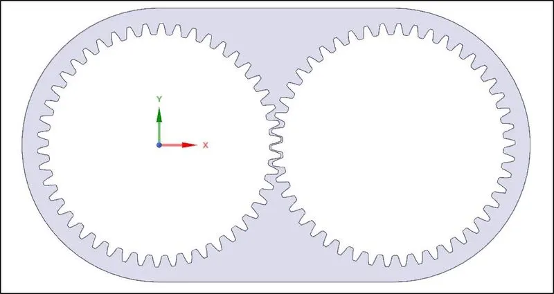
Fig. 1: Fluid Volume Model

2.2 Meshing

The meshing approach adopted for the given computational domain was developed to maintain the meshing quality attributes viz., element quality, skewness, orthogonality, and aspect ratio within the ranges as laid out in the Meshing training material of ANSYS outlined in the following table:

Element Quality			0 (Bad Mesh)	1 (Good Mesh)
Aspect Ratio		Triangles	1 (for an equilateral triangle)	- Best possible value
		Quadrilaterals	1 (for a square)	- Best possible value
Skewness	0-0.25 (Excellent)	0.25-0.50 (Very Good)	0.50-0.80 (Good)	0.80-0.94 (Acceptable)	0.95-0.97 (Bad)	0.98-1.00 (Unacceptable)
Orthogonal Quality	0-0.001 (Unacceptable)	0.001-0.14 (Bad)	0.15-0.20 (Acceptable)	0.20-0.69 (Good)	0.70-0.95 (Very Good)	0.95-1.00 (Excellent)

Table 1: Mesh Quality Attributes as defined in the ANSYS meshing training material

The reason for targeting the above mentioned mesh quality attributes comes from analysis across different types of geometries/models that these are few of the known ways of identifying whether the discretized mesh would face convergence issues during the solution process and also to locate areas in the mesh where the statistics can be improved. Named selections were created for edges corresponding to each gear so as to assign the required rotational motion, based on the UDF properties, also mentioned in Section 2.3.4. In Section 2.4.1, we will discuss in detail about the different meshes that were prepared and their mesh qualities.

2.3 CFD Simulation Setup, Material Definitions, UDF and Dynamic Mesh Setup, and Monitoring Points and Solution

The simulations on all meshes was performed using the Reynolds Averaged Navier-Stokes (RANS) models, in this case, the k-`epsilon` turbulence models and the VOF Multiphase models. The use of k-`epsilon` turbulence models and more specifically the k-`epsilon` Realisable turbulence model is attributed to the fact that the Reynolds number, based on the given flow conditions, lies in the turbulence flow region, explained in Section 2.4.2 Evaluation of Reynolds number. For the given modelling configuration, the multiphase flow regime represents that of a stratified/free-surface flow identified as a result of the flow of immiscible fluids separated by a distinctly clear interface. Based on the clarity of the multiphase flow regime, the VOF Multiphase model is best suited for the given numerical analysis. Additionally, all simulations were run using the double-precision feature as a general measure to resolve large variations in pressure differences. A brief description into the working of the k-`epsilon` turbulence model and VOF Multiphase model is provided below:

2.3.1 k-`epsilon` turbulence model

The k-`epsilon` turbulence model is one of the first RANS turbulence models proposed by Launder and Spalding and is still being widely used for its robust, economic approach and reasonable accuracy in simulation of mean flow characteristics of large number of industrial flows and heat transfer applications. The k-`epsilon` turbulence model consists of two transport equations, one for the turbulent kinetic energy (k) to evaluate the energy in turbulence and the other is for the turbulent dissipation (`epsilon`) to calculate the rate of dissipation of turbulent kinetic energy (k). In this particular simulation, we will be performing simulations using the Realisable k-`epsilon` model. The difference between the Realisable k-`epsilon` and standard k-`epsilon` model can be described in the following two ways:

1. The turbulent viscosity term is formulated differently in the Realisable k-`epsilon` model.
2. The dissipation rate `epsilon` in the transport equation has been modified and developed from the exact equation for transport of mean-square vorticity fluctuation.

The Realisable k-`epsilon` turbulence model is able to satisfy some of the mathematical constraints of the Reynolds's stresses such as the positive values of normal stresses when the eddy viscosity definition is used in the Boussinesq relationship and Schwarz inequality for shear stresses even when the main strain rate is large which otherwise would be negative. These formulations in the Realisable k-`epsilon` turbulence model have made them more popular to use over the other k-`epsilon` turbulence models especially when flow features include the presence of strong streamline curvature, vortices, and rotation.

2.3.1.1 Setup of the Realisable k-`epsilon` turbulence model:

To use the Realisable k-`epsilon` turbulence model in the Fluent component system, we navigate to Viscous option in Models under the Physics Tab. In the Viscous Model feature, we choose k-`epsilon` (2 eqn) Model with type set to 'Realisable' and Near Wall treatment as 'Enhanced Wall Treatment' so as to achieve accuracy of standard two-layer approach for near wall meshes while also not reducing the same when the mesh is coarse (also referred to as wall function meshes).

2.3.2 VOF Multiphase model

The VOF model, as mentioned before, is a surface-tracking technique employed when flow takes places between two immiscible fluids separated by an interface. The model makes use of a single set of momentum equations, shared by the fluids, with the volume fraction of each fluid computed and tracked in individual cells throughout the domain. The VOF formulation assigns a variable in the form of volume fraction of phases depending on the number of phases involved such that the sum of volume fractions of all phases equals to unity and also that the phases involved are not interpenetrating. This subsequently also leads to the respective fields for all variables and properties to be shared by the phases thereby creating volume-averaged values depending on the volume fraction of each phase at a given location.

2.3.2.1 Setup of the VOF Multiphase model

To use the VOF model in the Fluent component system, we navigate to Multiphase option in Models under the Physics Tab. In the Multiphase Model window, we choose Volume of Fluid under Homogeneous Models, Implicit Formulation under Volume Fraction Parameters and Sharp Type as Options for Interface Modeling as the setup configuration. It should be noted that Volume of Fluid model is only available under the Homogeneous Models section which implies that the phases in the domain are assumed to move with the same velocity, as is commonly assumed for free surface flows, and that all phases share all of the field variables except for volume fraction.

2.3.3 Material Definitions and Monitoring Points Setup

For the given problem, the materials and their properties used for defining the fluid and different types of lubricating oil, in combination, can be summarised in the following table:

Material Names	Density (`(kg)/(m^-3)`)	Viscosity (`(kg)/(m-s)`)
Air	1.225	`1.7894*10^(−5)`
Engine oil	889	1.06
n-heptane (`C_7H_16`)	684	0.000409

Table 2: Materials and their respective properties used in simulating the fluid-lubricating oil combination around the gears of the given computational domain

Since, the above mentioned materials, except air, are not present by default as an option from the Fluent Fluid Materials drop-down list, the same can be added by accessing the Fluent database, and searching and selecting the required lubricating oils, one at a time, followed by clicking on the 'Copy' and then the 'Close' buttons.

2.3.4 UDF, Dynamic Mesh and Cell Registers setup

The UDF created for the dynamic motion of the gears, similar to every other UDF, contains the following code structure:

1. Include statement for udf header file (identified by the extension 'h' in "udf.h") at the very beginning of the source code to allow definitions for Macros and functions to be part of the compilation process.
2. UDFs should be defined using DEFINE Macros furnished by Fluent.
3. UDFs also have access to data from the Fluent solver by making use of predefined macros and functions provided by Fluent.

As the UDF provided, 'rate.c', is a compiled UDF implying they are built similar to the Fluent executable. The process involves the use of a script called "Makefile" that invokes the C compiler of the system to build an object code library which with respect to the graphical user interface (GUI) can be performed by using the 'Build' button in the Compiled UDFs window found in the second option of the 'Functions' drop-down menu in the 'User Defined' section under the 'User Defined' tab. The shared library is then loaded at runtime into Fluent by the process of "dynamic loading" which from the GUI perspective is enabled by clicking on the load button in the same Compiled UDFs window.

Dynamic mesh model can be enabled by checking the 'Dynamic Mesh' checkbox available in the Dynamic Mesh Task Page which can be viewed by choosing 'Dynamic Mesh' option under the 'Mesh Models' drop-down menu of the 'Domain' tab. There are three sets of methods defining the manner in which the volume mesh may be updated in deforming zones based on the motion prescribed at the boundaries viz., Smoothing, Layering or Dynamic Layering and Remeshing.

Smoothing methods are incorporated to adapt the mesh in the zone corresponding to a moving or deforming boundary such that the interior nodes move, however, the total number of these nodes and its connectivity is retained, resembling the boundary movement is absorbed by the interior nodes. Smoothing methods can be further classified into three types i.e., Spring/Laplace/Boundary Layer, Diffusion and Linearly Elastic Solid. In diffusion based smoothing, diffusion equation governs the motion of the mesh with the diffusion coefficient controlling the behaviour of the boundary motion that in turn affects the interior mesh motion. The diffusion coefficient can be defined based on either Boundary Distance or the Cell Volume formulation with the former dependent on the normalised boundary distance such that diffusivity decreased away from the moving boundary leads to more absorption of the mesh motion with an attempt to preserve mesh quality near that boundary while the latter dependent on the normalised cell volume decreases diffusivity in larger cells directing them to absorb more of the mesh motion and striving to retain the cell quality of smaller cells. For the given numerical analysis, diffusion based smoothing is adopted, also considered as an alternative to spring based smoothing as it is applicable for all element types and can be utilised for updating mesh motion of moving or deforming boundaries and it can be activated by selecting the 'Diffusion' option from the 'Smoothing' method in the 'Mesh Method Settings' window. Despite being more computationally expensive than spring based smoothing, the results in mesh quality are significantly better as well as larger deformations are allowed before eventually breaking down. Additionally, the diffusion coefficient in this numerical problem is based on boundary distance as the motion of the gears are inherently rotational, with value of diffusion parameter set at 1.5 for the same reason and is also recommended as a good starting point by ANSYS Fluent which can be viewed by clicking on the 'Advanced' button in the 'Mesh Method Settings' window. AMG Stabilisation is set to conjugate gradient (CG) method by default and is considered to be faster than the other methods primarily because symmetry of the matrix utilised in linear systems of equations of finite-element based mesh smoothing is taken advantage, however, if divergence is noticed during the solution process, then the method switches to generalised minimal residual (GMRES) to improve linear solver robustness. 'Maximum number of iterations', 'Relative Convergence Tolerance' and 'Verbosity' are maintained at their default values of 50, 1e-10 and 0 respectively.

Dynamic Layering method adds or subtracts cells along layers in the neighbouring areas of the moving boundary based on the height of the layer and is typically used for hexahedral and/or wedge mesh zones in three-dimensional aspect or quadrilaterals in two-dimensional. In respect to the meshing strategy adopted for the given computational problem, as is also highlighted in Section 2.5 Meshing strategy, and time step size and total number of iterations calculations, the type of cells used are triangles (2D problem) and hence, dynamic layering method is not selected as a mesh motion method.

Remeshing methods is included in the Dynamic mesh model when displacement of the boundary is large in comparison to the cell size of the domain tending to deteriorated cell quality by grouping those cells that fail to comply with the skewness or sizing requirement and locally remeshing them. The remeshed cells, however, are not updated unless they met with the same skewness or sizing criteria and accordingly are either discarded or maintained. Thus, remeshing methods serve as an added benefit to a mesh smoothing method, typically used together, to prevent getting invalidated mesh that may lead to convergence issues during solution updation. For the given numerical analysis, remeshing option is opted by checking the option in the 'Dynamic Mesh' task page and local cell method, available in the 'Remeshing Methods Sizing Options' of the 'Remeshing' tab in the 'Mesh Method Settings' window, was opted as the Remeshing method. Local cell remeshes grid that are triangular and tetrahedral cell type while other cell types remain unaffected, which based on the meshing strategy mentioned in Section 2.5 Meshing strategy, and time step size and total number of iterations calculations, makes it applicable. Additionally, cells are remeshed on the basis of the limiting values outlined in the 'Parameters' section of the 'Remeshing' tab in the 'Mesh Method Settings' window which includes minimum and maximum length scale values (in m), maximum cell skewness and size remeshing interval. In the case of all remeshing parameters for the given computational problem, maximum length scale was selected as the mesh element size, minimum length scale was chosen to be a value of order one less than the smallest element size, maximum cell skewness was maintained at 0.95 (with 0.98 being recommended by ANSYS Fluent) and size remeshing interval was retained at 5 by default. These values can also be referenced with respect to a particular mesh by accessing the 'Default' button in the same window. Therefore, the remeshed local cells need to ensure that the new skewness value is less than the maximum cell skewness, new minimum length scale is smaller than that mentioned as its limiting value and new maximum length scale is larger than its specified value in the list of 'Parameters' in the 'Remeshing' tab of the 'Mesh Method Settings' window.

For the dynamic mesh model to be implemented at run time, regions of the model need to be identified wherein the dynamic motion is present which in this case is specified at the left and right gears respectively. As both the gears represent rigid body motion (all points on both the gears are experiencing same angular velocity at all times), both dynamic mesh zones were created of the type rigid body, set under 'Type' section of the 'Dynamic Mesh Zones' window with zone names set accordingly. Since, the compiled UDF was loaded, each gear could be assigned its motion as defined in the UDF , however, the 'Center of Gravity location' for the left gear from the CAD model in SpaceClaim was centered at the origin while the right gear was offset at a distance of 0.115m in the positive x-axis direction.

In order to visualise the flow field and especially along the interface between the fluid and the lubricating oil in the computational domain, a surface needs to be developed which is done by creating a cell register wherein the cells are grouped by region. A surface, in two-dimensional numerical problem, also aids in creation of XY plots, adapting the mesh, and reporting on the cells among its many advantages. A region type of cell register allows marking of cells inside or outside of the given region, in this case, being inside. Since, the immersion values represents the amount of lubricating oil in which the gears are placed, region cell registers are defined based on a quadrilateral shaped area with respect to the height of lubricating oil from the bottom of the enclosure i.e., the bottom part of the quadrilateral represents the starting or initial level of lubricating oil while the height upto which the gears are immersed represents the top part and the points defining the diagonal with minimum and maximum of X and Y coordinates of the formed quadrilateral are recorded.

Immersion (%)	X Min (m)	X Max (m)	Y Min (m)	Y Max (m)
20	-0.05706	0.17208	-0.0675	-0.03595
30	-0.06304	0.17808	-0.0675	-0.02395

Table 3: Immersion (%) values and corresponding coordinates of the formed quadrilateral cell register region

2.3.5 Solution

The nature of given CFD simulation is transient while type of solver chosen is Pressure-based solver as we are dealing with a low-speed incompressible flow problem i.e., speed of fluid flow is typically in the subsonic range and density of material does not change or the change is almost negligible within the given control volume, although the Fluent Theory Guide also claims that the Pressure-based solver can now solve and operate beyond its previous limitations. Also, a steady-state VOF calculation is not possible as inflow boundaries are not present and the solution is not independent of initial conditions, which implies with respect to the initial level of lubricating oil and fluid in the domain. The Pressure-based solver calculates the Pressure field by evaluating the pressure or pressure-correction equation that is determined from the manipulation of continuity and momentum equations. Velocity formulation is chosen to be absolute as the velocity in the given fluid control volume is not rotating. Since, the movement of lubricating oil and fluid mixture was influenced by the gravitational field, 'Gravity' option was enabled with y-axis as the reference direction and value in Y set to -9.81 `m/s^2` representing downward direction of gravitational acceleration on the system. Plots to monitor the static pressure and volume fraction of selected lubricating oil for the numerical analysis were created to observe the fluctuations in these properties with regards to the gear motion and to draw inferences when errors such as 'Dynamic mesh failed' error or 'Negative cell volume detected' error that could occur during the solution process. To create the required monitoring plots, we head over to the 'Definitions' drop-down menu in the 'Reports' section of the 'Solution' tab and choose 'Area-Weighted Average' option in the 'Surface Report' followed by assigning the name as static pressure or volume fraction, depending on the monitor plot, choosing 'Pressure' or 'Phases' in the 'Field Variable', 'Static Pressure' or 'Volume Fraction' as the attributes, 'Mixture' or 'lubricating-oil' as 'Phase', selecting all surfaces in the 'Wall Zones' list, checking the 'Report File' and 'Report Plot' boxes before clicking on the 'OK' button. To run the solution, the given fluid volume needs to be initialised which in this case is done using the Hybrid Initialisation option for a similar reason of not having defined inlet and/or outlet zones as was mentioned earlier in the case of not being able to use a steady state VOF setup. Hybrid Initialisation as described in the Fluent Theory Guide solves a Laplace equation to create a velocity flow field that will adhere to the domain geometry and a pressure field across the same domain to allow smooth transition of high and low pressure values. In the given computational analysis, the use of Hybrid Initialisation was combined with Patch option to assign the volume fraction values to lubricating oil phase as 1 while also ensuring the cell register is also selected during the process. A contour plot to depict the movement of lubricating oil relative to the gears, as a function of time, during the simulation run and recorded as a MPEG animation file was setup. The contour plot was now available to be created under the 'Graphics' section of the 'Results' tab since the solution was initialized. After a new contour plot option was selected from the 'Contours' drop-down menu, a name was assigned, in this case, 'vof-lubricating oil', followed by clicking on the 'Filled' check-box, choosing 'Phases' as the field variable with 'Volume Fraction' as the attribute and setting 'Phase' to the selected lubricating oil defined during the material definition before clicking on the 'Save/Display' button. An animation plot of the same contour was created by heading back to the 'Solution' tab and clicking on the 'Solution Animations' option available under the 'Create' drop-down menu of the 'Activities' section. In the 'Animation Definition' window, the name of the animation was assigned as 'vof-lubricating-oil-animation' and 'vof-lubricating-oil' was chosen which was the name of the contour plot before clicking on 'OK'. Additionally, during the entire run, the default convergence criteria values were unaltered for 'continuity', 'x-velocity', 'y-velocity', 'k', '`epsilon`' and 'vf-lubricating oil' as tabulated in Table 8. The definition of run calculation activities were based around the time step size, number of time steps and maximum iterations per time step.

2.4 Meshing strategy, Reynolds number estimation and time step size and total number of iterations calculations

In this numerical simulation two different mesh sizes were prepared and time step size and total number of iterations were evaluated based on them, both of which have been discussed in detail in Section 2.4.1 Baseline and Refined Meshes and Section 2.4.2 Determination of transient parameters respectively.

2.4.1 Baseline and Refined Meshes

A baseline mesh for the given computational domain was created with an element size of 0.0075m, illustrated in Fig. 2, using the 'All Triangles Method' to create cell type of triangles throughout the domain. The 'All Triangles Method' was chosen due to the profile shape of the gear teeth which would otherwise be difficult for a higher quality cell type, such as quadrilateral shaped cells, to occupy as well as to ensure consistency with minimum number of highly skewed cells. Additionally, 'Capture Proximity' in 'Sizing' was set to 'Yes' with 'Num Cells Across Gap' maintained at value of 1. Proximity based sizing feature along with 'Num Cells Across Gap' was chosen to control the minimum number of element layers especially in the spaces between the two gears.

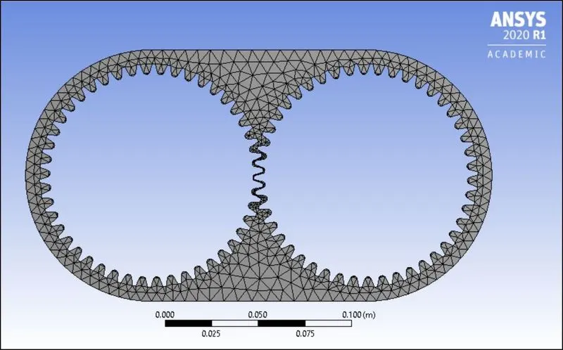
Fig. 2: Baseline Mesh

Mesh statistics and quality attributes for Baseline Mesh:

Mesh	Element-Size(m)	Nodes	Elements	Element Quality(avg.)	Aspect Ratio(avg.)	Skewness(avg.)	Orthogonal Quality(avg.)
Baseline	0.0075	1066	1360	0.8519	1.7158	0.21502	0.86053

Table 4: Mesh statistics and quality attributes for Baseline Mesh

A Refined mesh following the same description as that of the Baseline mesh was created, only this time the element size was changed to a value of 0.0025m, with Fig. 3 highlighting the same and Table 5 representing its statistics and quality attributes.

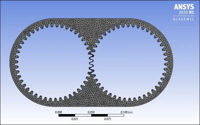
Fig. 3: Refined Mesh

Mesh statistics and quality attributes for Baseline Mesh:

Mesh	Element-Size(m)	Nodes	Elements	Element Quality(avg.)	Aspect Ratio(avg.)	Skewness(avg.)	Orthogonal Quality(avg.)
Refined	0.0025	2257	3430	0.95118	1.2424	7.0651e-002	0.95542

Table 5: Mesh statistics and quality attributes for Refined Mesh

Comparing the two meshes i.e., the Baseline Mesh and the Refined Mesh, it can be seen that the latter offers better average quality attributes over the former as the cells look more uniform and evenly distributed across the domain.

2.4.2 Evaluation of Reynolds number

Critical Reynolds number for splash lubricated gears based on the individual churning gear loss model proposed by Changenet et. al [2, 3] and dimensional drag group based on dimensional analysis using the Vashy-Buckhingam theorem can be expressed mathematically as:

`Re_c = (R_p*b*omega)/nu`; where (Eq. 1)

`R_p` is the Pitch Radius (in m),

`b` represents Tooth Face Width, and

`omega` is the angular velocity (in rad/s), and

`nu` is kinematic viscosity (in `m^2/s`)

`R_p` is determined from the pitch diameter, D, which can be evaluated from the following mathematical expression:

`D = (N*p)/pi`; where (Eq. 2)

`N` refers to the number of teeth, which in this case is same on both the left and right gear and is found out to be 46, and

`p` points to the circular pitch which is the distance measured from a point on one gear tooth to the same point on the adjacent gear tooth along the circumference of the Pitch Diameter. The pitch diameter is the diameter of the pitch circle which refers to an imaginary circle that will contact with the pitch circle of the gear it is to be meshed. The circular pitch from SpaceClaim was evaluated to be 7.89mm or 0.00789m. Therefore, pitch diameter resulted in a value of 0.1155m and pitch radius subsequently becomes 0.05755m. Also, since this is a two-dimensional numerical analysis, the value of tooth face width which represents the length of the gear teeth in the axial plane is assumed to be unity.

Substituting the value of pitch radius, tooth face width and omega equal to 200 rad/s (from UDF, 'rate.c'), the values for critical Reynolds number (`Re_c`) is tabulated as shown below:

Lubricating Oil	Kinematic Viscosity (`nu`)[`mu/rho`] (From Table 2)	Critical Reynolds number (`Re_c`) (Eq. 1)
Engine oil	`1.192*10^-3`	9656.04
n-heptane (`C_7H_16`)	`5.98*10^-7`	19247491.64

Table 6: Kinematic Viscosity (`nu`) and critical Reynolds number (`Re_c`) for Engine Oil and n-heptane (`C_7H_16`)

Since the values reported for the critical Reynolds number for both the Engine oil and n-heptane (`C_7H_16`) in Table 6 is greater than 4000, it can be inferred that the flow lies in the turbulent regime. It should be noted that the accuracy of the calculated values of critical Reynolds number is dependent on the accuracy of the model and the prevailing conditions under which the said fluid is exhibiting flow properties.

2.4.3 Determination of transient parameters

Value of angular velocity based on the definition of DEFINE_CG_MOTION macro for both the left and right gear motions in the compiled UDF 'rate.c' is given as 200 rad/s in directions opposite to each other identified by the signs assigned to the values. Therefore, rotational speed of gears in revolutions per minute (rpm) can be evaluated mathematically as shown below:

`omega = (2*pi*N)/60`; where (Eq. 3)

'N' is the rotational speed (in rpm)

From Eq. 3, we get value of N as 1909.86 rpm which is also equivalent to 31.831 revolutions per second (rps) or for 1 revolution to occur, the time taken is 0.0314s. In order to understand the fluid flow behaviour within the Academic license restrictions, it was decided to perform transient analysis for a minimum of 2 gear revolutions or for a total flow time of 0.0628s. Time-step size and total number of time steps was decided based on the Courant-Friedrichs-Lewy Condition or the CFL number which is expressed below:

`CFL = (u*Delta t)/(Delta x)`; where (Eq. 4)

`Delta t` is time-step size,

`Delta x` represents the length scale a particular mesh, in this case, the mesh element size, and

`u` is linear velocity which, in this case, is evaluated from the angular velocity defined in the UDF as:

`omega = u/R_p` or `u = omega*R_p`, where (Eq. 5)

Therefore `u` from Eq. 5 results in a value of 11.51m/s. Total number of time steps can now be calculated as:

`T = 0.0628/(Delta t)` (Eq. 6)

Since, an implicit transient formulation was being used for the given numerical analysis, the CFL criteria was limited to a value of 2. The values of time-step size and number of total time-steps from Eq. 4 and Eq. 6 respectively, as seen in Table 7, were then utilised to define the run calculations.

Mesh	`Delta x` (in m)	Time-step size (`Delta t`) (Eq. 4)	Total number of time steps (`T`) (Eq. 6)
Baseline	0.00043742	`7.6007*10^-5`	~827
Refined	0.00043742	`7.6007*10^-5`	~827

Table 7: Time-step size (`Delta t`) values and Total number of time steps for Baseline and Refined Meshes

The above calculated values of time-step size and total number of time steps reflects the transient formulation based on the initial mesh length scale, however, as was reported in Section 2.3.4 UDF, Dynamic Mesh and Cell Registers setup, the smallest element size during remeshing could reach an order less than that reported as `Delta x` in Table 7, depending on other parameters. Hence, the time-step size for Baseline Mesh was altered to `5*10^-5` with total number of time steps as 1300, while for Refined Mesh the time-step size was changed to `1*10^-5` with total number of time steps as 6300 and these values were decided also with regards to limitations on computational resources.

2.5. Convergence Level

In the given numerical analysis, Pressure based solver of type SIMPLE scheme was utilised. SIMPLE scheme by definition is iterative in nature, robust (memory efficient) and is quicker per iteration than other pressure-based solvers. The selection of schemes for the different terms under spatial discretization includes assigning Gradient to Least Squares Cell Based scheme, Pressure to PRESTO! scheme, Momentum to first order upwind scheme, Volume Fraction to Compressive scheme, Turbulent Kinetic Energy to first order upwind scheme and Turbulent Dissipation Rate to first order upwind scheme. For Transient Formulation, the scheme was set to First Order Implicit. Least Squares Cell Based scheme is the default gradient method chosen by ANSYS Fluent which is used to compute the change in values across the centroid of two cells along a vector path and is a computationally less expensive scheme offering comparable accuracy to the node-based gradient scheme, both of which are superior to the cell-based gradient scheme. PRESTO! scheme, which stands for PREssure STaggering Option, is the default scheme for pressure spatial discretization when the VOF Multiphase model is enabled and it makes use of a discrete continuity balance for a "Staggered" control volume about the face to compute the required pressure on it and is generally considered to indicate physically accurate results as it avoids interpolations and the associated errors due to it. First order upwind scheme for the momentum term was made use of owing to the maximum skewness varying based on the remeshing settings, which as the name of the scheme suggests is of first order accuracy as it assumes the cell centre values of the field variables to be computed represents cell average values that hold good across a cell as the quantity to be determined at the cell face. Compressive scheme for the Volume Fraction spatial discretization uses a second order reconstruction scheme which is evaluated based on the value of the slope limiter and is dependent on the type of interface regime modelling selected for a numerical analysis. Slope limiters prevents the occurrence of spurious oscillations or wiggles that are otherwise bound to be generated when using spatial discretizations of higher order. Compressive scheme is also applicable for the given analysis as the meshes generated are of good quality and yields better accuracy when compared against Modified HRIC in most cases as these two schemes are the only options available based on the configuration selected. The turbulence terms viz., Turbulent Kinetic Energy and Turbulent Dissipation Rate are set at first order upwind scheme by default which makes use of quantities at the cell faces as the cell-average value indicating that it is first-order accurate. The reason to have the turbulence terms discretized using the first-order upwind scheme is based on observations from simulations across different applications when using a higher or even second order upwind scheme leads the computational cost to become more expensive (more compute time) solution while also demonstrating stability issues in the form of repeating oscillations of values and not necessarily guaranteeing always a more accurate solution. The selection of First Order Implicit scheme for Transient Formulation was done primarily to observe the movement of the fluid-lubricating oil combination and the gear motion using large time-step sizes despite it tending to produce more numerical diffusion when compared to either the Second Order Implicit or Bounded Second Order Implicit schemes as a result of limitations in computational resources. Convergence criteria option was retained and the residual values which measures the local imbalance of conserved variable in each control volume such as continuity, x-velocity, y-velocity, k, `epsilon`, and engine oil or n-heptane liquid depending on the lubricating oil selected were monitored throughout the solution process for the defined number of time steps to allow the development of the fluid behaviour. The residual limits defined for the k-`epsilon` turbulence model and VOF Multiphase model equations and the residual plots corresponding to the different meshes, immersion values, remeshing settings and adoption of higher order discretization for momentum are shown in the table and figures below:

	k-`epsilon`	VOF Multiphase
continuity	1e-03	--
x-velocity	1e-03	--
y-velocity	1e-03	--
k	1e-03	--
`epsilon`	1e-03	--
vf-engine-oil	--	1e-03
vf-n-heptane	--	1e-03

Table 8: Residual Values of the different equations used in the Realisable k-`epsilon` turbulence and VOF Multiphase models

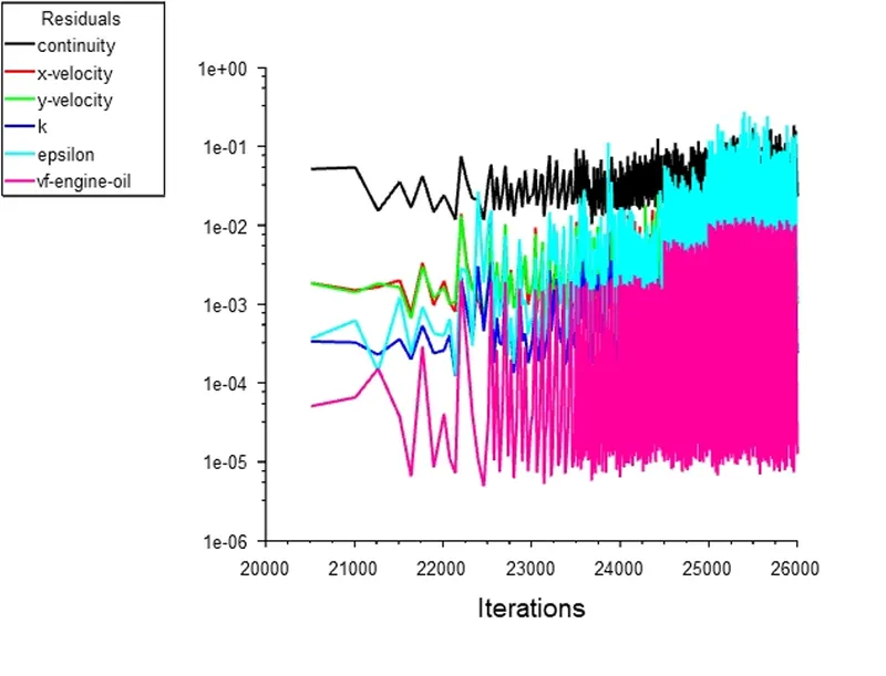
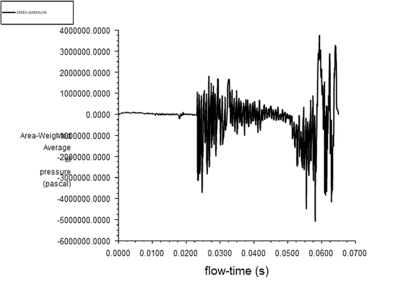
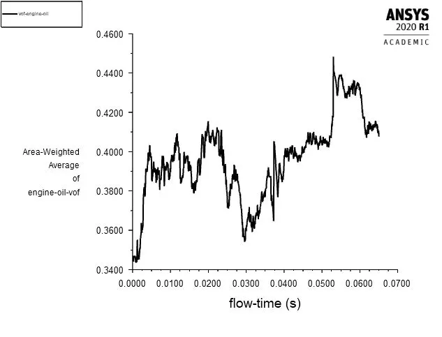
Fig. 4: Scaled Residuals, Static Pressure and Volume Fraction plots for Air - Engine oil combination with 20% immersion configuration using the Realisable k-`epsilon` turbulence model for baseline mesh with SIMPLE solver

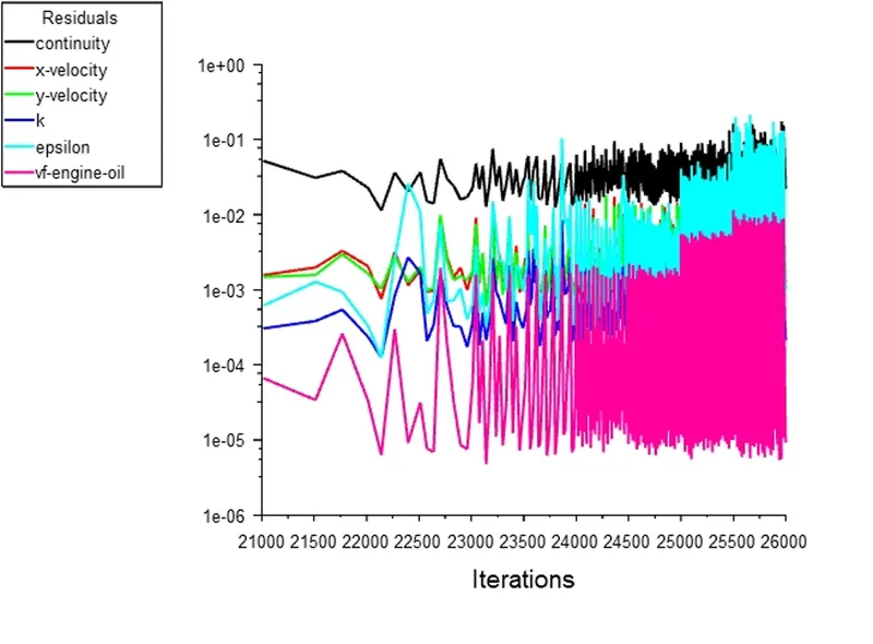
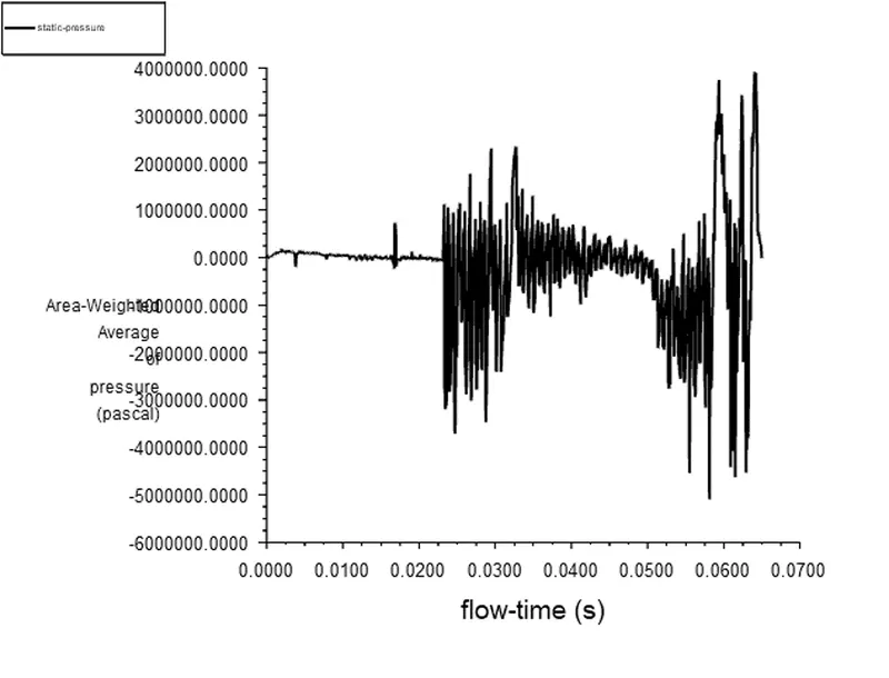
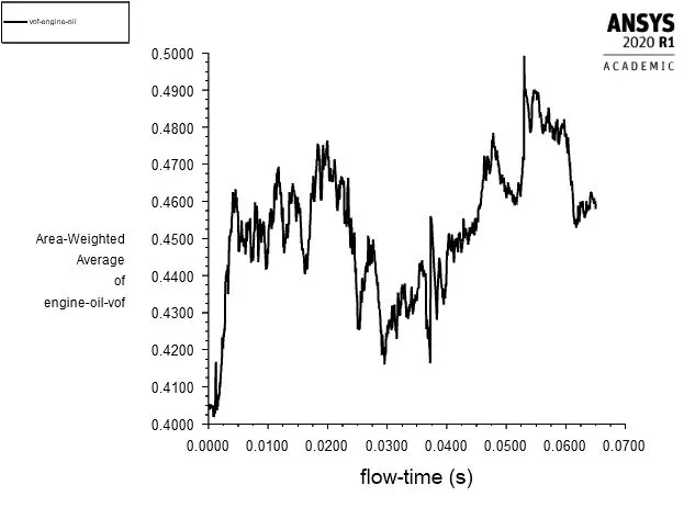
Fig. 5: Scaled Residuals, Static Pressure and Volume Fraction plots for Air - Engine oil combination with 30% immersion configuration using the Realisable k-`epsilon` turbulence model for baseline mesh with SIMPLE solver

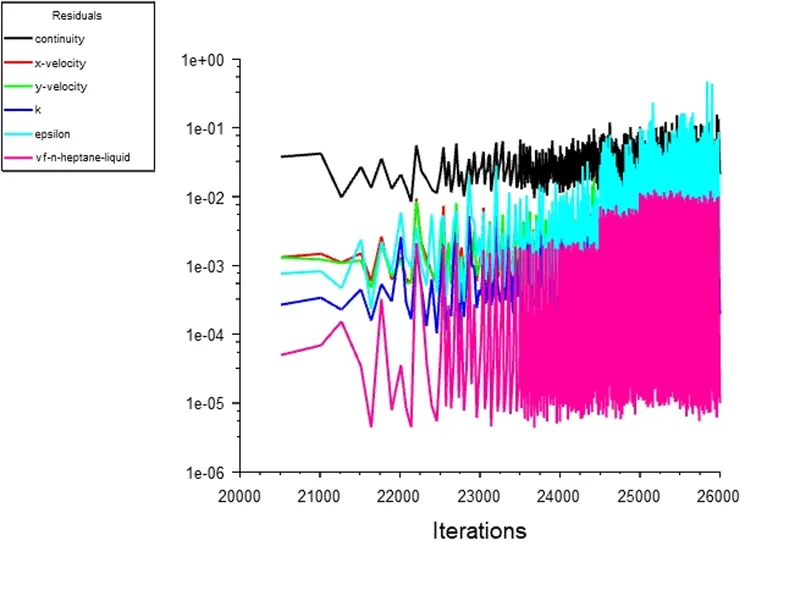
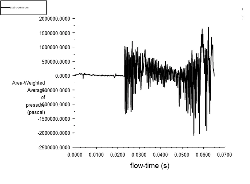
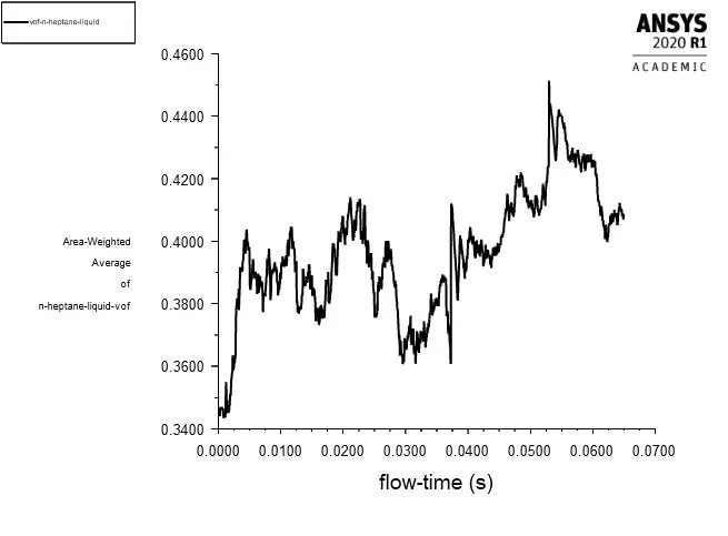
Fig. 6: Scaled Residuals, Static Pressure and Volume Fraction plots for Air-n-heptane (`C_7H_16`) combination with 20% immersion configuration using the Realisable k-`epsilon` turbulence model for baseline mesh with SIMPLE solver

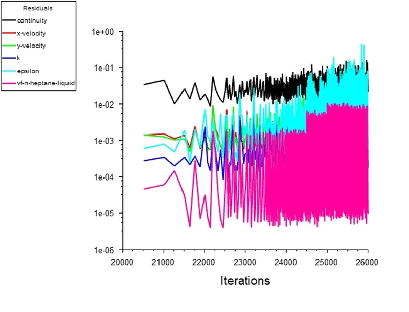
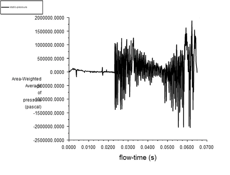
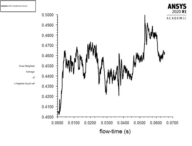
Fig. 7: Scaled Residuals, Static Pressure and Volume Fraction plots for Air-n-heptane (`C_7H_16`) combination with 30% immersion configuration using the Realisable k-`epsilon` turbulence model for baseline mesh with SIMPLE solver

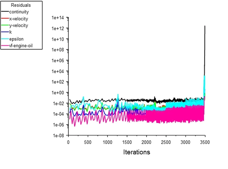
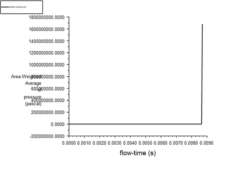
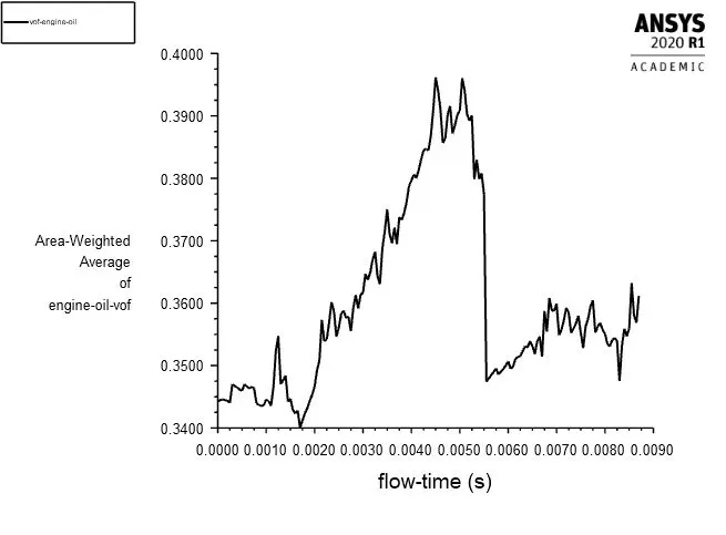
Fig. 8: Scaled Residuals, Static Pressure and Volume Fraction plots for Air - Engine oil combination with 20% immersion configuration using the Realisable k-`epsilon` turbulence model for baseline mesh with SIMPLE solver and second order upwind spatial discretization scheme for momentum

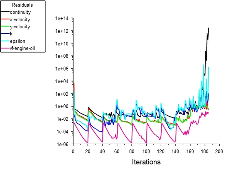
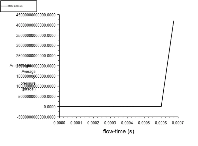
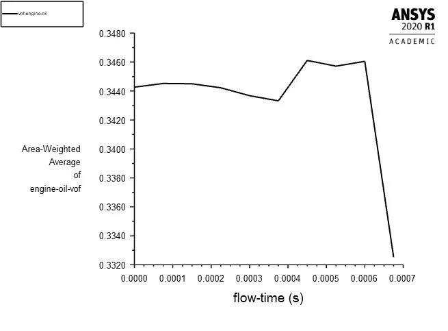
Fig. 9: Scaled Residuals, Static Pressure and Volume Fraction plots for Air - Engine oil combination with 20% immersion configuration using the Realisable k-`epsilon` turbulence model for baseline mesh with SIMPLE solver and time step size value increased to 7.5e-5s

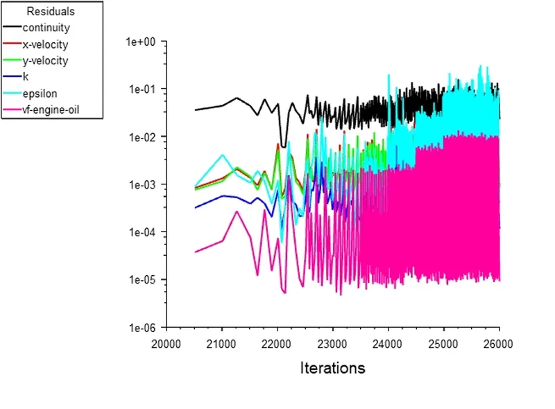
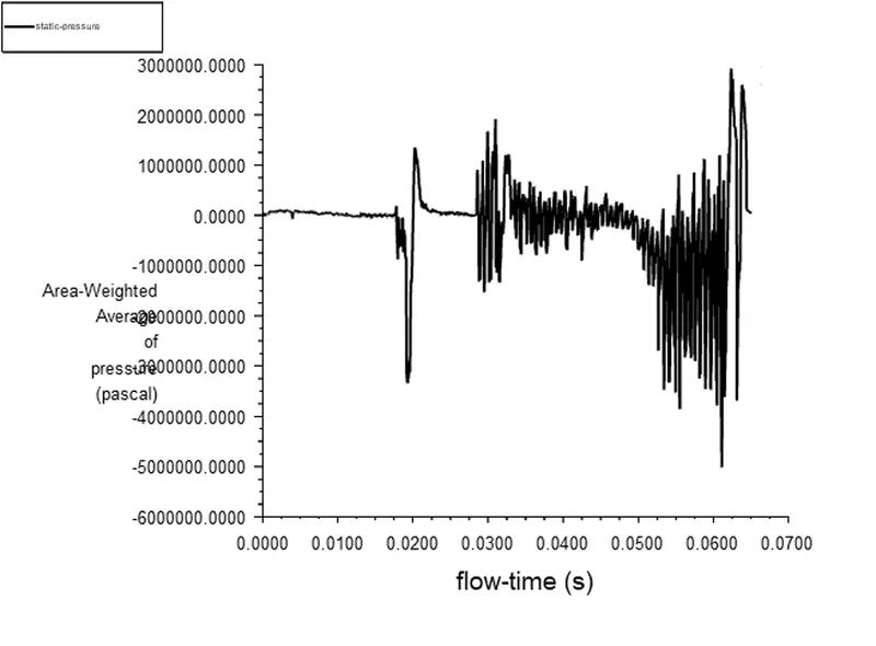
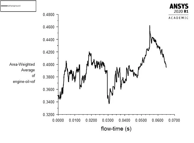
Fig. 10: Scaled Residuals, Static Pressure and Volume Fraction plots for Air - Engine oil combination with 20% immersion configuration using the Realisable k-`epsilon` turbulence model for baseline mesh with SIMPLE solver and meshing interval value changed to 3

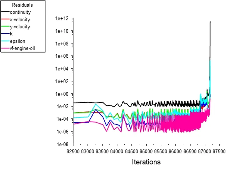
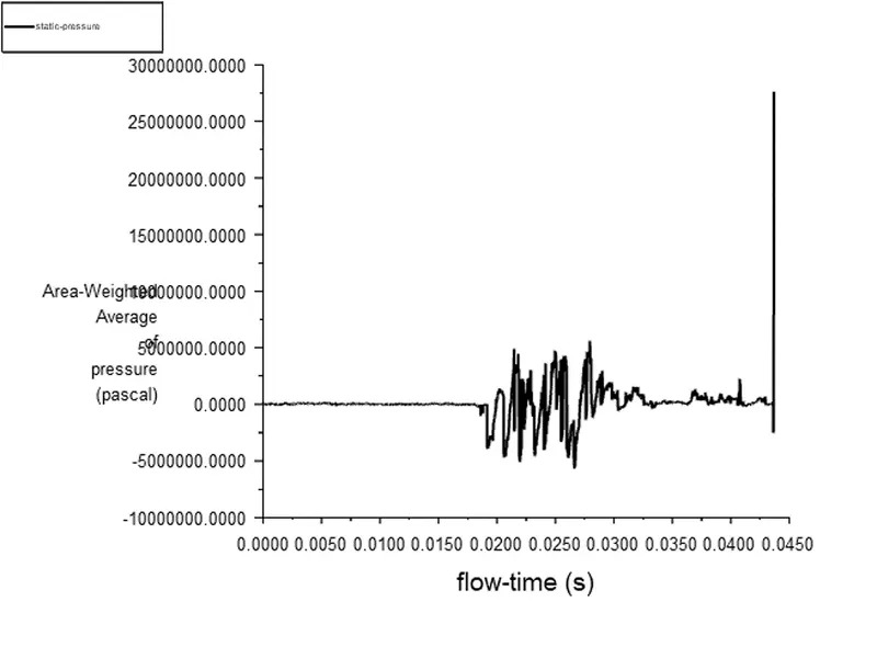
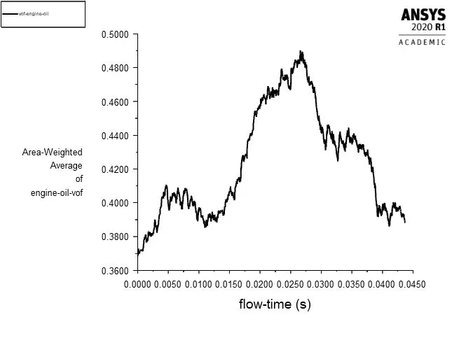
Fig. 11: Scaled Residuals, Static Pressure and Volume Fraction plots for Air - Engine oil combination with 20% immersion configuration using the Realisable k-`epsilon` turbulence model for refined mesh with SIMPLE solver

From Fig. 4, Fig. 5, Fig. 6 and Fig. 7, we can notice the transient behaviour of the fluid-lubricating oil undergoing volume fraction changes and pressure variations in their respective monitor plots across the computational domain as well as a distinctly clear pattern in the residuals being recorded and while continuity equations show difficulty in reaching for convergence as they are well above the '1e-03' default limit, they continue to oscillate between the '1e-01' and '1e-02' limits. This implies that for more number of max iterations per time step than the default 20, the continuity equations could oscillate at even lower residual values, however, due to constraints on computational resources, the value was left unchanged. Fig. 8 and Fig. 9 display residual and monitor plots for pressure and volume fraction when second order discretization for momentum was selected and time-step size value was increased respectively and it can be deduced that the given mesh configuration made it difficult to achieve more accurate results in the case of higher order spatial discretization and that the CFL condition was violated as velocity of flow during initial iterations were still low leading to 'Negative cell volume detected' error in both cases. Thus, one way of identifying 'Negative cell volume detected' error, in this case, is by locating the extent to which the mesh has moved in a single time step leading the cells to collapse. Fig. 10, like Fig. 4 and Fig. 5 showed similar trends in reporting residual values and monitor plot behaviours only this time with remeshing taking place at every third interval as opposed to fifth and while variations in results were hard to trace for the given mesh setup, a more refined mesh may add better clarity to the same. In Fig. 11, similar to Fig. 8 and Fig. 9, a 'Negative cell volume detected' error was observed towards a flow time of approximately 0.0450s implying that the time-step size selected for the transient behaviour needed to be further reduced which was again difficult to achieve due to limited computational resources. The other type of error that arose during one of the simulation trials using parallel processing as opposed to single processing was 'floating point exception' error which indicates that the solver attempts to compute arithmetic operations, such as division by zero or numbers exceeding their bounds with respect to the defined data types and in either case leading to divergence of solution. This issue can be dealt by making use of under-relaxation factors or reducing time step size or refining the mesh as few of the commonly employed troubleshooting options.

3. Results and Discussion

In Section 3.1, numerical simulation results with regards to the fluid-lubricating oil movement across the computational domain using different lubricating oils are compared and discussed.

3.1 Numerical results for fluid-lubricating oil movement across the computational domain using different lubricating oils

3.1.1 Effect of different immersion depths

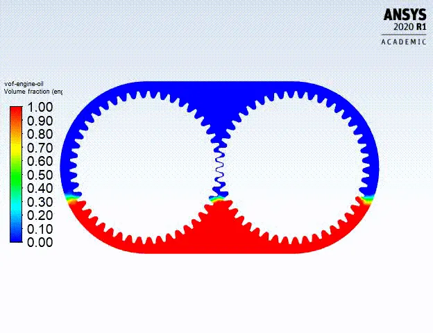
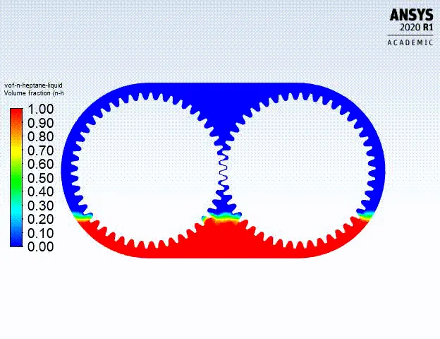
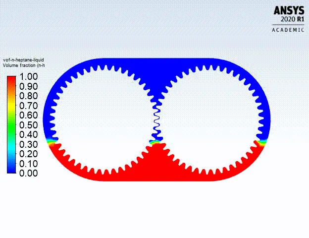
In both cases of lubricating oils, engine oil and n-heptane liquid, the spacing between the teeth on each gear as well as adjacent gears are initially lubricated earlier with greater immersion depth as can be seen in Fig. 12 and Fig. 13, however, the effects of splashing and the subsequent length of the same also significantly increases as long as the gears are in motion. Due to splashing for a prolonged period combined with the sloshing effect on the gearbox, the gears may experience loss of lubrication for brief moments of time which is unfavourable to the operation and service life especially in critical applications including in the marine industry. Additionally, churning losses are an inherent drawback in splash lubricated gearboxes which refers to the force required to churn through the lubricating oil and these interactions are commonly observed between the gear and the lubricating oil as well as between the mating gears at the interface along with squeezing and pocketing losses dominating at these locations. As immersion depths keep rising, the possibilities for a hydraulic lock also tends to increase due to excessive lubrication.

3.1.2 Effect of different lubricating oils

From Table 2, it is evident that engine oil is heavier and more viscous than n-heptane liquid and therefore implies that engine oil as a lubricating oil may produce better film thickness, however, churning losses may also be significantly greater. Thus, in situations where high temperature persists either on the external boundaries of the housing or is produced internally as a result of the concerned gear operations, engine oil as a lubricating medium may be preferred whereas lower viscosity lubricating oil is generally used in constant speed, load, and temperature conditions as a cheaper alternative to higher viscosity lubricating oils.

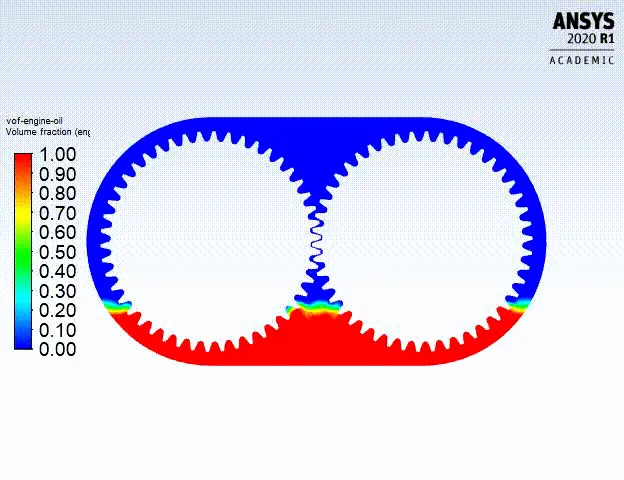
a) Air and Engine Oil (phase materials) - 20% immersion b) Air and Engine Oil (phase materials) - 30% immersion

Fig. 12: Movement of fluid-lubricating oil with Air and Engine Oil as phase materials at different immersion percentage values for Baseline Mesh

a) Air and n-heptane-liquid (phase materials) - 20% immersion b) Air and n-heptane-liquid (phase materials) - 30% immersion

Fig. 13: Fluid-lubricating oil movement with Air and n-heptane-liquid as phase materials at different immersion percentage values for Baseline Mesh

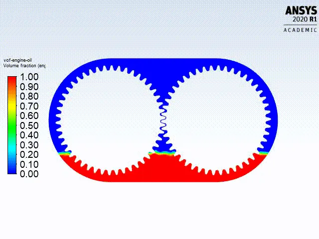
Fig. 14: Movement of fluid-lubricating oil with Air and Engine Oil as phase materials at 20% immersion for Refined Mesh

4. Conclusion

The numerical analysis for movement of fluid-lubricating oil within a gearbox housing domain with air and different lubricating oils as phases under transient conditions using the realisable k-`epsilon` turbulence model and VOF Multiphase model in ANSYS Fluent 2020 R1 was well understood. The impact of dynamic mesh model along with a UDF defining the gear motion allowed for a more realistic impression of splash lubrication system that is employed in many important applications. Moreover, the immersion depth and type of lubricating oil contribute immensely to the efficiency of not only the lubrication technique but also the gearbox performance. In regards to the changes with the setup for observing the transient behaviour of the fluid-lubricating oil combination within the gearbox computational domain gave significant insight into the role played by each parameter and its effects on the solution and its performance.

5. References

[1] ANSYS Fluent Theory Guide, Release 2020 R1 - © ANSYS, Inc. All rights reserved.

[2] C. Changenet, G. Leprince, F. Ville, and P. Velex, A Note on Flow Regimes and Churning Loss Modeling, Journal of Mechanical Design 133 (2011), no. 12, 121009.

[3] P. Marques, Efficiency of a Gearbox Lubricated with Wind Turbine Gear Oils, Master's Degree Dissertation, Faculdade de Engenharia da Universidade do Porto, 2012