Gate Valve Parametric Study
1. Introduction
Gate valves can be described as a type of device, in the form of a gate or wedge shaped disc, that operates perpendicularly to the direction of fluid flow passing through a given channel or piping configuration to offer regulated movement of the said fluid. The highlight feature of a gate valve assembly construction is an almost uninterrupted flow of fluid through the passageway thereby leading to minimal pressure drop across the setup. This characteristic marks great use in applications such as oil and gas industries, manufacturing and automotive to name a few. The given gate valve model, as an overview, consists of a handwheel, spindle (also known as stem), the gate disc, bonnet and seat on either side of the main body. Handwheel connected to the spindle allows for the more often linear motion of the gate disc. Bonnet protects the contained internal moving parts of the assembled model and can be removed at different intervals to perform the necessary maintenance and/or replacement activities of the different components. Gate valve assemblies vary in configurations and are often classified based on the types of disk, types of body bonnet joint and types of stem movement. Advantages of gate valve assemblies include use of different media like slurries and viscous fluids, bi-directional flow, easier maintenance and disassembly, relatively inexpensive, available in large sizes, operational as a shut-off valve and usually fire-safe for metal sheet based construction. Drawbacks are limitations on lower pressure values, operational time is slow either during opening or closing, disk and seat erosion depending on the prevalent conditions, poor throttling features, repair of parts are difficult and is best avoided in sanitary based applications.
The aim of this challenge is to perform steady-state simulations of the given gate valve model with fluid passing through the piping configuration being water at 10 pascals as the gauge total pressure at the inlet in order to determine the mass flow rate at the outlet, and flow coefficient and flow factor values by varying the valve lift positions for different valve opening configurations from 10% to 80%. Moreover, a graph was also plotted to provide the necessary inference for flow coefficient and flow factor at each opening of the valve.
2. Method
2.1 Modelling
The computational domain for simulating flow of fluid viz., water, within the given gate valve configuration was modelled in SpaceClaim, the default solid modeling CAD software for the Fluid Flow (Fluent) Analysis System. The position of the gate disc within the bottom and bonnet components of the gate valve assembly controlled the passage of water from the inlet to the outlet sections. As the current setting of the gate disc ensured no water could pass through, the gate disc was required to be moved to its initial placement of 10% opening away from its locked location, or in this case 10mm in the positive z-axis direction of its global coordinate system as both the inlet and outlet sections through which water was allowed to travel corresponded to 100mm in diameter, using the "Move" tool in the 'Edit' menu of the 'Design' tab and subsequently this dimension was parameterised by clicking on the letter/icon "P" that appeared after the numerical value was selected and/or entered. Also, as the inlet and outlet areas did not specify well-defined lengths for pipes, those ends of the bottom component were extruded in either direction by utilising the "Pull" tool, found in the same location as that of the "Move" tool, to values of 800mm each. The inlet, outlet and the zone occupying the space above the gate disc to the upper surface limit of the bottom component are identified and marked as regions representing the entry, movement and exit of water respectively corresponding to the Fluid Volume domain which was subsequently created using the "Volume Extract" option in the 'Edit' menu of the 'Prepare' tab, while remaining regions were suppressed for discretization and physics as they are solid structures that are not part of any analysis being performed, however, the bottom, gate disc and the spindle components were not hidden as the Fluid Volume domain was required to adapt based on the volume body in context depending on the positioning of the gate disc. This implied that although the extents of the Fluid Volume domain remained the same, the Fluid Volume shape or structure changed based on the amount of opening for the passage of water controlled by the gate disc. Moreover, the extruded regions of the inlet and outlet areas, with regards to the bottom component, no longer required to be recreated as the domain was originally extended to its pre-determined limits of 800mm mentioned earlier. Although, the extracted Fluid Volume is symmetrical about the XZ axial plane, it was decided to use the entire model for discretization and solution of the partial differential equations which will be discussed in detail regarding the setup in subsequent sections.

Fig. 1: Fluid Volume Model and Boundary Conditions regions (D = 0.1m represents pipe inlet and outlet diameters, and length of gate valve in cross flow direction)
2.2 Meshing
The meshing approach adopted for the given computational domain was developed to maintain the meshing quality attributes viz., element quality, skewness, orthogonality, and aspect ratio within the ranges as laid out in the Meshing training material of ANSYS outlined in the following table:
|
Element Quality |
0 (Bad Mesh) |
1 (Good Mesh) |
||||
|
Aspect Ratio |
Triangles |
1 (for an equilateral triangle) |
- Best possible value |
|||
|
Quadrilaterals |
1 (for a square) |
- Best possible value |
||||
|
Skewness |
0-0.25 (Excellent) |
0.25-0.50 (Very Good) |
0.50-0.80 (Good) |
0.80-0.94 (Acceptable) |
0.95-0.97 (Bad) |
0.98-1.00 (Unacceptable) |
|
Orthogonal Quality |
0-0.001 (Unacceptable) |
0.001-0.14 (Bad) |
0.15-0.20 (Acceptable) |
0.20-0.69 (Good) |
0.70-0.95 (Very Good) |
0.95-1.00 (Excellent) |
Table 1: Mesh Quality Attributes as defined in the ANSYS meshing training material
The reason for targeting the above mentioned mesh quality attributes comes from analysis across different types of geometries/models that these are few of the known ways of identifying whether the discretized mesh would face convergence issues during the solution process and also to locate areas in the mesh where the statistics can be improved. For each of the mesh, named selections such as inlet and outlet were created so as to assign their respective boundary conditions in the setup stage. Also, depending on the name of the named selection, Fluent is able to assign an inlet or outlet boundary condition with pressure-inlet and pressure-outlet type boundary conditions respectively which is a useful feature to have in flow-type problems of similar nature since the user now can only add values relating to the specific boundary condition thereby making the setup process a lot faster. In Section 2.5.3, preparation about the different meshes have been discussed in detail along with their mesh qualities and the arrival on mesh independent solution.
2.3 CFD Simulation Setup, Boundary Conditions, Monitoring Points and Solution
The simulations on all meshes was performed using the Reynolds Averaged Navier-Stokes (RANS) models, in this case, the k-`epsilon` turbulence model. The use of k-`epsilon` turbulence models and more specifically the Realisable k-`epsilon` turbulence model is attributed to the fact that the Reynolds number, based on the given flow conditions, lies in the turbulence flow region, explained in Section 2.5.1 Evaluation of Reynolds number. Additionally, all simulations were run using the double-precision feature as a general measure to resolve large variations in pressure differences. A brief description into the working of the k-`epsilon` turbulence model is provided below:
2.3.1 k-`epsilon` turbulence model
The k-`epsilon` turbulence model is one of the first RANS turbulence models proposed by Launder and Spalding and is still being widely used for its robust, economic approach and reasonable accuracy in simulation of mean flow characteristics of large number of industrial flows and heat transfer applications. The k-`epsilon` turbulence model consists of two transport equations, one for the turbulent kinetic energy (k) to evaluate the energy in turbulence and the other is for the turbulent dissipation (`epsilon`) to calculate the rate of dissipation of turbulent kinetic energy (k). In this particular simulation, we will be performing simulations using the Realisable k-`epsilon` model. The difference between the Realisable k-`epsilon` and standard k-`epsilon` model can be described in the following two ways:
- The turbulent viscosity term is formulated differently in the Realisable k-`epsilon` model.
- The dissipation rate `epsilon` in the transport equation has been modified and developed from the exact equation for transport of mean-square vorticity fluctuation.
The Realisable k-`epsilon` turbulence model is able to satisfy some of the mathematical constraints of the Reynolds's stresses such as the positive values of normal stresses when the eddy viscosity definition is used in the Boussinesq relationship and Schwarz inequality for shear stresses even when the main strain rate is large which otherwise would be negative. These formulations in the Realisable k-`epsilon` turbulence model have made them more popular to use over the other k-`epsilon` turbulence models especially when flow features include the presence of strong streamline curvature, vortices, and rotation.
2.3.1.1 Setup of the Realisable k-`epsilon` turbulence model:
To use the Realisable k-`epsilon` turbulence model in the Fluent component system, we navigate to Viscous option in Models under the Physics Tab. In the Viscous Model feature, we choose k-`epsilon` (2 eqn) Model with type set to 'Realisable' and Near Wall treatment as 'Scalable Wall Functions' as wall bounded effects for the given flow conditions were deemed as not of high significance and that the wall function displaces the mesh to a `y^+` value of 11.225 which lies in the transition of the log-law composite region, regardless of the levels of refinement, and thereby preventing modelling errors of the laminar sub-layer and buffer regions.
2.3.2 Boundary Conditions and Monitoring Points
The different boundary conditions for the simulation of flow of water within the gate valve model is described in the following table:
|
Named Selections |
inlet |
outlet |
wall |
|
Type |
pressure-inlet |
pressure-outlet |
wall |
|
Direction Specification Method |
Normal to Boundary |
-- |
-- |
|
Gauge Total Pressure (pascal) |
10 |
-- |
-- |
|
Supersonic/Initial Gauge Pressure (pascal) |
0 |
-- |
-- |
|
Turbulence Specification Method |
Intensity and Viscosity Ratio |
Intensity and Viscosity Ratio |
-- |
|
Turbulent Intensity (%) |
5 |
-- |
-- |
|
Turbulent Viscosity Ratio |
10 |
-- |
-- |
|
Pressure Profile Multiplier |
-- |
1 |
-- |
|
Backflow Direction Specification Method |
-- |
Normal to Boundary |
-- |
|
Gauge Pressure (Pa) |
-- |
0 |
-- |
|
Backflow Pressure Specification |
-- |
Total Pressure |
-- |
|
Backflow Turbulent Intensity (%) |
-- |
5 |
-- |
|
Backflow Turbulent Viscosity Ratio |
-- |
10 |
-- |
|
Wall Motion |
-- |
-- |
stationary wall |
|
Shear Condition |
-- |
-- |
no slip |
Table 2: Boundary Conditions for simulation of flow of water within the given gate valve assembly setup
For the given problem, the material properties for the fluid is changed to water with density value of 998.2 `(kg)/m^3` and the viscosity (or dynamic viscosity) value of `1.003*10^(−3) (kg)/(ms)` by accessing the Fluent database. The material as water flowing through the fluid control volume can be verified by heading over to the "volume_volume" zone of "Cell Zones" under the "Zones" section of the "Physics" tab and click on "Edit" button for viewing the different attributes of the same.
The choice of Turbulence specification method chosen for this simulation is Intensity and Viscosity Ratio wherein the Intensity (or Turbulent Intensity) is defined as the ratio of root-mean-square (RMS) value of velocity fluctuations to average flow velocity while Viscosity Ratio (or Turbulent Viscosity Ratio) is defined as the ratio of the turbulent viscosity to the laminar viscosity. Turbulent intensity is set to a value of 5% (representing medium intensity) and the Turbulent Viscosity Ratio has its default value at 10 since this value was not directly available from any experimental findings and in that case these values usually lie in a typically good scale or range as is recommended in the lecture series by ANSYS on Turbulence Modeling.
During the solution process, the mass flow rate plots was monitored at the outlet to observe stability in its value. The required monitoring plot was created from the 'Definitions' drop-down menu in the 'Reports' section of the 'Solution' tab and choosing 'Mass Flow Rate' item in the 'Flux Report', 'Mass Flow Rate' as the option in the 'Options' section of the 'Flux Report Definition' window followed by selecting outlet as the boundary from the 'Boundaries' list, checking the 'Report File', 'Report Plot' and 'Create Output Parameter' boxes before clicking on the 'OK' button. The 'Create Output Parameter' option allows visualisation of mass flow rate as the output variable to the parametric study without creating a separate Fluent analysis system in ANSYS Workbench enabling easier setup of different cases using different design points with the input variable defined during the "Move" tool operation as a result of clicking on the letter/icon "P" in Section 2.1 Modelling. Fig. 1 outlines the named selections where the boundary conditions would be employed as well as gradient plots to demonstrate the velocity and static pressure distributions discussed in Section 2.3.3 Solution.
2.3.3 Solution
The nature of given CFD simulation is steady while type of solver chosen is Pressure-based solver as we are dealing with a low-speed incompressible flow problem i.e., speed of fluid flow is typically in the subsonic range and density of material does not change or the change is almost negligible within the given control volume, although the Fluent Theory Guide also claims that the Pressure-based solver can now solve and operate beyond its previous limitations. The Pressure-based solver calculates the Pressure field by evaluating the pressure or pressure-correction equation that is determined from the manipulation of continuity and momentum equations. Velocity formulation is chosen to be absolute as the velocity in the given fluid control volume is not rotating. Since, the gate disc is present within the valve body which contains a curved region extending below the level of the lower surface of both the inlet and outlet pipes, fluid medium, in this case water, needs to undergo change in its travel along the vertical distance as a result of the potential energy head which is influenced by the gravitational field, therefore 'Gravity' option was enabled with z-axis as the reference direction and value in Z set to -9.81 `m/s^2` representing downward direction of gravitational acceleration on the system. To run the solution, the given fluid volume needs to be initialised, which in this case is done using the 'Standard Initialisation' option. Standard Initialisation, as described in the Fluent Theory Guide, allows the user to specify all the variables directly as initial guess values across each cell of the entire domain. The variables can include initial guess values for velocity, temperature, pressure, etc. from the available list. In this case, the flow field is initialised by utilising the values set at the 'Inlet' in the 'Compute from' drop-down list with values corresponding to the same zone now available under the 'Initial Values' section. A contour plot to illustrate the static pressure and velocity magnitude gradients during the simulation run was setup along the mid plane in the YZ planar direction and further used to record as their subsequent MPEG animation files. Both, the creation of mid plane in the YZ axial direction and contour plots were now available to be created using the 'Create' and 'Contours' options under the 'Surface' and 'Graphics' sections of the 'Results' tab respectively since the solution was initialized. After a new contour plot option was selected from the 'Contours' drop-down menu, a name was assigned, in this case, 'static-pressure-contour' for 'Pressure' as the field variable with 'Static Pressure' as the attribute and similarly, 'velocity-contour' for 'Velocity' as the field variable with 'Velocity Magnitude' as the attribute, followed by clicking on the 'Filled' check-box and selecting the 'cut-plane-yz' in the 'Surfaces' list before clicking on the 'Save/Display' button. An animation plot of the same contours was created by heading back to the 'Solution' tab and clicking on the 'Solution Animations' option available under the 'Create' drop-down menu of the 'Activities' section. In the 'Animation Definition' window, the name of the animation was assigned as 'static-pressure-contour-animation' and 'velocity-contour-animation' with 'static-pressure-contour', and 'velocity-contour' chosen as the names of the contour plots respectively, on an individual basis, before clicking on 'OK'. Additionally, during the entire run, the default convergence criteria values were unaltered and disabled by selecting the 'Residuals' option in the 'Reports' section of the 'Solution' tab and unchecking the 'continuity', 'x-velocity', 'y-velocity', 'z-velocity', 'k', and '`epsilon`' for k-`epsilon` turbulence model to monitor the solution based on the number of iterations.
2.4 Post-Processing
In order to plot the velocity and static pressure gradient plots, velocity vectors, and streamlines across the domain length for the given fluid flow problem, Line and Plane locations at different positions in the gate valve assembly model were drawn. Legends have been added for vectors, streamlines and gradient plots for a better understanding of the graphical representation and can be viewed under Section 3 Results.
Expressions:
Pressure Inlet = areaAve(Pressure)@Plane Line 2
Pressure Outlet = areaAve(Pressure)@Plane Line 10
Pressure Drop = abs(Pressure Inlet - Pressure Outlet)
Definition of Lines at different distances along the spanwise flow direction (Refer Fig.1 indicated by yellow coloured lines):
Line 1 @0.7m from pipe inlet downstream:
|
Point |
x[m] |
y[m] |
z[m] |
|
Point 1 |
0 |
-0.123 |
-0.195 |
|
Point 2 |
0 |
-0.123 |
-0.095 |
Table 3: Definition of Line 1
Line 2 @0.77m from pipe inlet downstream:
|
Point |
x[m] |
y[m] |
z[m] |
|
Point 1 |
0 |
-0.053 |
-0.195 |
|
Point 2 |
0 |
-0.053 |
-0.095 |
Table 4: Definition of Line 2
Line 3 @0.793m from pipe inlet downstream:
|
Point |
x[m] |
y[m] |
z[m] |
|
Point 1 |
0 |
-0.03 |
-0.21 |
|
Point 2 |
0 |
-0.03 |
-0.155 |
Table 5: Definition of Line 3
Line 4 @0.803m from pipe inlet downstream:
|
Point |
x[m] |
y[m] |
z[m] |
|
Point 1 |
0 |
-0.02 |
-0.215 |
|
Point 2 |
0 |
-0.02 |
-0.155 |
Table 6: Definition of Line 4
Line 5 @0.813m from pipe inlet downstream:
|
Point |
x[m] |
y[m] |
z[m] |
|
Point 1 |
0 |
-0.01 |
-0.22 |
|
Point 2 |
0 |
-0.01 |
-0.155 |
Table 7: Definition of Line 5
Line 6 @0.823m from pipe inlet downstream:
|
Point |
x[m] |
y[m] |
z[m] |
|
Point 1 |
0 |
0 |
-0.225 |
|
Point 2 |
0 |
0 |
-0.155 |
Table 8: Definition of Line 6
Line 7 @0.833m from pipe inlet downstream:
|
Point |
x[m] |
y[m] |
z[m] |
|
Point 1 |
0 |
0.01 |
-0.22 |
|
Point 2 |
0 |
0.01 |
-0.155 |
Table 9: Definition of Line 7
Line 8 @0.843m from pipe inlet downstream:
|
Point |
x[m] |
y[m] |
z[m] |
|
Point 1 |
0 |
0.02 |
-0.215 |
|
Point 2 |
0 |
0.02 |
-0.155 |
Table 10: Definition of Line 8
Line 9 @0.853m from pipe inlet downstream:
|
Point |
x[m] |
y[m] |
z[m] |
|
Point 1 |
0 |
0.03 |
-0.21 |
|
Point 2 |
0 |
0.03 |
-0.155 |
Table 11: Definition of Line 9
Line 10 @0.876m from pipe inlet downstream:
|
Point |
x[m] |
y[m] |
z[m] |
|
Point 1 |
0 |
0.053 |
-0.195 |
|
Point 2 |
0 |
0.053 |
-0.095 |
Table 12: Definition of Line 10
Line 11 @0.946m from pipe Inlet downstream:
|
Point |
x[m] |
y[m] |
z[m] |
|
Point 1 |
0 |
0.123 |
-0.195 |
|
Point 2 |
0 |
0.123 |
-0.095 |
Table 13: Definition of Line 11
Definition of Planes at different distances along the spanwise and latitudinal flow direction:
Plane 1 at centre of the gate valve assembly model in the flow direction (Refer Fig.1 indicated by grey coloured plane):
Option = YZ Plane
Type = Slice
X = 0.0 [m]
Plane 2 at definition of Line 2:
Option = ZX Plane
Type = Slice
Y = -0.053 [m]
Plane 3 at definition of Line 10:
Option = ZX Plane
Type = Slice
Y = 0.053 [m]
Streamline plots are created using Type "3D Streamline" and 'Start From' selected as Line 2 and Line 10 respectively to visualise the flow profiles near the gate valve wherein the fluid undergoes change in its travel distance depending on the value of the valve displacement. In the streamlines definition, the "Variable" option is selected as "Velocity" and the option for "Cross Periodics" is checked on along with the "Forward" option under "Direction" drop-down retained for the first streamline (Line 2) and "Backward" option for the second streamline (Line 10).
Gradient plots that display the velocity and pressure variations across the fluid domain was created using the plane 1 definition as specified above with 'Colour Variable' representing velocity and pressure values respectively. For the gradient plot, the 'Range' was set to "Local" which was available under the 'Color' tab implying that the values of the concerned variable highlighted the maximum and minimum range values corresponding to the current time step, or in this case at the last iteration number.
Additionally, a vector plot to display velocity vector quantities was created using the Line definitions as mentioned from Table 3 to Table 13 along the spanwise flow direction with 'Reduction' option selected as 'Maximum Number of Points' and 'Max Points' set to 50 as was the number of 'Line Samples' designated during the line definitions, 'Normalized Symbols' using "Line Arrow" depiction and size of 0.15. The vector plot aids in enhancing the flow profile along the flow field direction as the "Line Arrow" symbols with their orientation indicate direction which implies that recirculation region will be demarcated by backward facing or cross-facing line arrows.
2.5 Reynolds number estimation, and Meshing strategy and Verification
In this numerical simulation, verification of calculation (or mesh independence study) was carried out based on comparison of the minimum percentage variation (%var) in the predicted values of the mass flow rate quantity, more of which has been highlighted in Section 2.5.3 Mesh Refinement approach.
2.5.1 Evaluation of Reynolds number
Turbulence characteristics for the governing flow conditions are determined based on the pipe flow Reynolds number and can be expressed as:
`Re = (rho*U*D)/mu`; where (Eq. 1)
`mu` is the dynamic viscosity of the fluid (in `(kg)/(m*s)`),
`rho` represents fluid density (in `(kg)/(m^3)`),
`D` is the pipe diameter (in m), and
`U` is inlet flow velocity (in m/s)
Substituting the inlet flow velocity obtained from the set of initial values during initialisation using the 'Standard Initialisation' option, pipe diameter, and density and dynamic viscosity of water with values of 0.1415m/s, 0.1m, and 998.2 `(kg)/m^3` and `1.003*10^(−3) (kg)/(ms)` respectively into (Eq. 1) we get the Reynolds number as 14082.283. Since the value for the Reynolds number is greater than the limit defining turbulence of 4000 for internal flow simulation, it can be inferred that the flow lies in the turbulent regime.
2.5.2 Baseline Mesh
A baseline mesh, illustrated in Fig. 2, for the given computational domain was created with default element size of 0.092892m. For the given numerical analysis, three different schemes viz., SIMPLE, SIMPLEC and COUPLED, were compared to understand the effect on convergence and stability of the residuals and static pressure monitor plots as they are preferred algorithms for solving steady-state numerical problems unlike PISO which is generally used for transient calculations with large time steps. A detailed description of each of the three schemes have been mentioned in Section 2.6 Convergence Level.
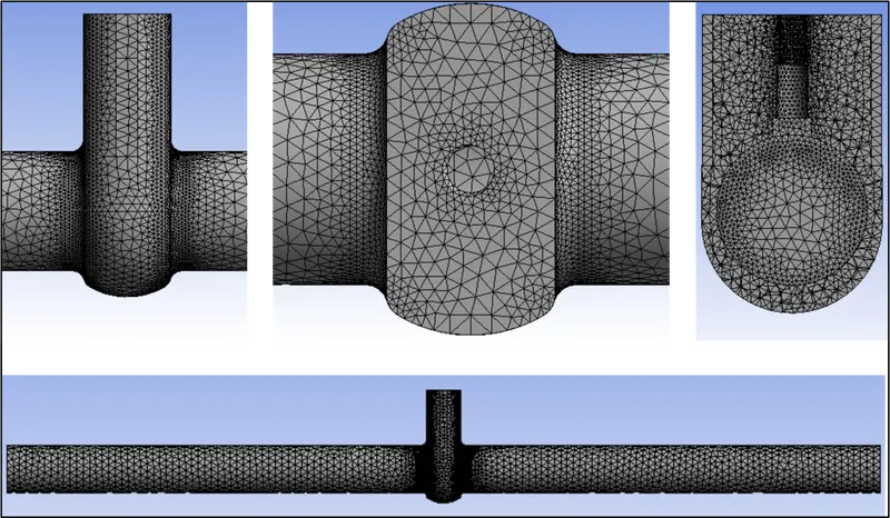
Fig. 2: Baseline Mesh
Mesh statistics and mass flow rate values at the outlet for Baseline Mesh using different Pressure-Velocity coupling schemes:
|
Mesh |
Mesh Element Size [m] |
Nodes |
Elements |
Pressure-Velocity Coupling Scheme |
Mass Flow Rate - Outlet [kg s^-1] |
|
Baseline |
0.092892 |
29198 |
137869 |
SIMPLE |
0.149003 |
|
Baseline |
0.092892 |
29198 |
137869 |
SIMPLEC |
0.149011 |
|
Baseline |
0.092892 |
29198 |
137869 |
COUPLED |
0.149034 |
Table 14: Mesh statistics and mass flow rate values at the outlet for Baseline Mesh using different Pressure-Velocity coupling schemes
Mesh quality attributes for Baseline Mesh:
|
Mesh |
Element Quality(avg.) |
Aspect Ratio(avg.) |
Skewness(avg.) |
Orthogonal Quality(avg.) |
|
Baseline |
0.82 |
Triangles-1.9317 |
0.25079 |
0.74743 |
Table 15: Mesh quality attributes depicting average values of element quality, aspect ratio, skewness and orthogonal quality for Baseline mesh of the gate valve model
2.5.3 Mesh Refinement approach
The initial results obtained from the Baseline mesh in Section 2.5.2 Baseline Mesh with regards to the convergence behaviour of the three different algorithms, SIMPLE, SIMPLEC and COUPLED, as can be seen in Fig. 7, Fig. 8, and Fig. 9 respectively, it was observed that all monitor plots demonstrated highly stable outputs well before they reach the total number of iterations of 500, however, the COUPLED solver performed better than the two previously stated algorithms with regards to achieving stable values for the mass flow rate monitor plot at the outlet based on minimum number of iterations required as well as in terms of reporting the lowest value of residuals, except maybe for the continuity term with almost similar range of values across all the schemes, as opposed to the convergence limits mentioned in Table 18 (although the convergence criteria option for all equations were checked off) making the results obtained more reliable and accurate for it to be reused to solve the pressure-velocity equations for the four different meshes that were prepared to obtain a mesh independent solution. It is important to note that the maximum skewness reported for the Baseline Mesh by Fluent was 0.98291, which is more than the recommended value of 0.98 (highly skewed cells lead to convergence difficulties, decreased accuracy and unstable solution), and while results with SIMPLE and SIMPLEC schemes may have varied for a mesh with reduced skewness, the purpose of the Baseline Mesh was to guide towards an improved mesh refinement strategy that ensured not only the underlying physics was well captured but also the results were at least in close proximity to the default convergence criteria. The mesh refinement hereafter was created, while adhering to the mesh quality attributes mentioned in Section 2.2 Meshing, with the mesh element size being reduced by 20% and 'Capture Curvature' and 'Capture Proximity' options set to 'Yes' due to the presence of many curvature bound regions and small gaps including the number of cells across gap adjusted to a value of 1, in every subsequent mesh iteration, to minimize errors due to numerical diffusion that eventually led to uniform division of the meshing elements and consequently reduced skewness.
Mesh 1:
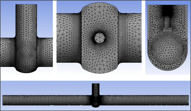
Fig. 3: Mesh 1
Mesh 2:
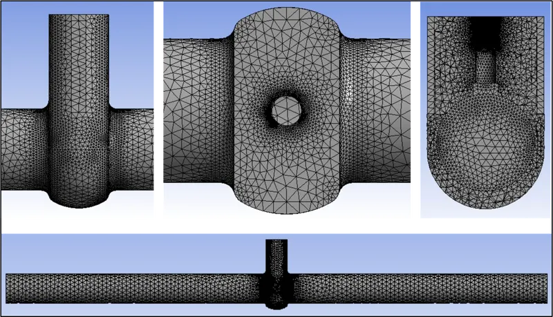
Fig. 4: Mesh 2
Mesh 3:
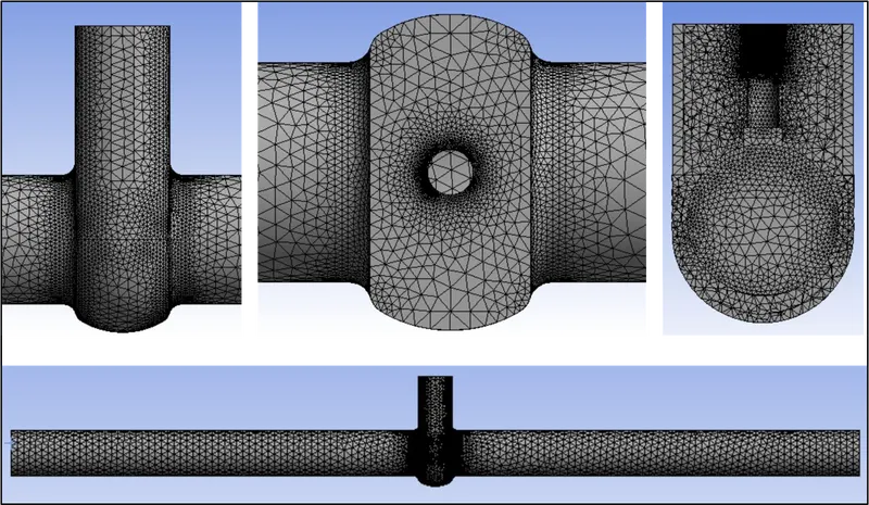
Fig. 5: Mesh 3
Mesh 4:
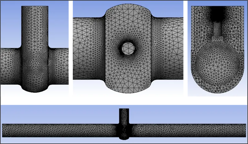
Fig. 6: Mesh 4
Mesh statistics and mass flow rate values at the outlet for different meshes using COUPLED Pressure-Velocity coupling scheme:
|
Mesh |
Mesh Element Size [m] |
Nodes |
Elements |
Mass Flow Rate - Outlet [kg s^-1] |
%var |
|
1 |
0.02472 |
90185 |
468229 |
0.14884 |
-- |
|
2 |
0.0206 |
90394 |
469200 |
0.14877 |
-0.0470 |
|
3 |
0.017196 |
90785 |
471058 |
0.14869 |
-0.0538 |
|
4 |
0.01433 |
92606 |
479821 |
0.14865 |
-0.0269 |
Table 16: Mesh statistics, mass flow rate values for different meshes at the outlet using COUPLED Pressure-Velocity coupling scheme and its minimum percentage variation values with subsequent mesh
Mesh quality attributes for the four different meshes:
|
Mesh |
Element Quality(avg.) |
Aspect Ratio(avg.) |
Skewness(avg.) |
Orthogonal Quality(avg.) |
|
1 |
0.83537 |
Triangles - 1.8514 |
0.23119 |
0.76737 |
|
2 |
0.83546 |
Triangles - 1.851 |
0.23112 |
0.76746 |
|
3 |
0.83545 |
Triangles - 1.8508 |
0.23129 |
0.76729 |
|
4 |
0.83584 |
Triangles - 1.8493 |
0.23072 |
0.76784 |
Table 17: Mesh quality attributes depicting average values of element quality, aspect ratio, skewness and orthogonal quality for different meshes of the gate valve model
From the meshing statistics in Table 16, mesh number 3 (or mesh 3) with 471058 elements represents a mesh independent result in terms of minimum percentage variation (%var) in the predicted values of mass flow rate quantity at the outlet. The %var is calculated as the ratio of the difference of the predicted values in two consecutive meshes to the predicted value of the previous mesh e.g., ((Mass Flow Rate at outlet for Mesh 2 - Mass Flow Rate at outlet for Mesh 1)/Mass Flow Rate at outlet for Mesh 1). Due to constraints in computational resources and limitations in maximum number of cells/nodes for solution by ANSYS Student license to 512,000 any further reduction in values of mesh element size was not possible to achieve for the given numerical analysis. On a closer look, it is difficult to observe noticeable differences in external areas of the different meshes prepared as seen from Fig. 3 to Fig. 6, as the meshing algorithm based on the values defining the 'Capture Curvature' and 'Capture Proximity' options allows almost similar number of cells to be occupied in those regions, however, refinement is carried out in other areas of the Fluid Volume and to a certain degree near the gate valve location which can be visualised in the sectional views of the same. Results in Section 3 will only be referred with regards to the mesh independent solution i.e., Mesh 3.
2.6 Convergence Level
As mentioned earlier in Section 2.5.2 Baseline Mesh, three different schemes i.e., SIMPLE, SIMPLEC and COUPLED were compared with regards to convergence study. SIMPLE scheme is iterative in nature, robust (memory efficient) and is quicker per iteration than other pressure-based solvers. SIMPLEC scheme, similar to the SIMPLE scheme, allows increased under relaxation to the pressure correction term that improves in convergence times especially when employed in complicated flows with turbulence and/or supplementary physical models and as such offers greater diversity in terms of computational problems for implementation over SIMPLE scheme. While SIMPLE and SIMPLEC schemes are segregated type of schemes i.e., pressure and velocity terms are updated sequentially, the COUPLED scheme on the other hand updates the pressure and velocity terms simultaneously. This allows the COUPLED scheme to be more efficient in its single-phase implementation especially for steady-state flows offering superior performance over the segregated algorithms (SIMPLE and SIMPLEC) thereby requiring fewer iterations to converge. The selection of schemes for the different terms under spatial discretization includes assigning Gradient to Least Squares Cell Based scheme, pressure to second order scheme, momentum to second order upwind scheme, and Turbulent Kinetic Energy and Turbulent Dissipation Rate to the first order upwind scheme. Least Squares Cell Based scheme is the default gradient method chosen by ANSYS Fluent which is used to compute the change in values across the centroid of two cells along a vector path and is a computationally less expensive scheme offering comparable accuracy to the node-based gradient scheme, both of which are superior to the cell-based gradient scheme. The second order scheme for the pressure makes use of the central differencing scheme and is generally considered to be more accurate than the Standard and Linear schemes as well as robust in the case of skewed meshes. A second order upwind scheme is chosen for the momentum term that makes use of the quantities at the cell face values to compute a cell-centered solution at the cell centroid leading to a second order accurate solution. The turbulence terms viz., Turbulent Kinetic Energy and Turbulent Dissipation Rate are set at first order upwind scheme by default which makes use of quantities at the cell faces as the cell-average value indicating that it is first-order accurate. The reason to have the turbulence terms discretized using the first-order upwind scheme as was noted in observations from simulations across different applications is because using a higher or even second order upwind scheme leads to a computationally expensive (more compute time) solution while also demonstrating stability issues in the form of repeating oscillations of values and not necessarily guaranteeing always a more accurate solution. Convergence criteria option was checked off, however, the residual values which measures the local imbalance of conserved variable in each control volume such as continuity, x-velocity, y-velocity, z-velocity, k, and `epsilon` were monitored throughout the solution process for the defined number of iterations i.e., 500, to allow for the development of the flow behaviour which is the flow of water across the gate valve assembly. The residual limits defined for the turbulence model equations, and the residual and monitor plots corresponding to the different meshes are shown in the table and figures below respectively:
|
k-`epsilon` |
|
|
continuity |
1e-03 |
|
x-velocity |
1e-03 |
|
y-velocity |
1e-03 |
|
z-velocity |
1e-03 |
|
k |
1e-03 |
|
`epsilon` |
1e-03 |
Table 18: Residual Values of the different equations used in the Realisable k-`epsilon` turbulence model
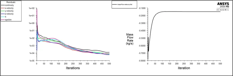
Fig. 7: Scaled Residuals and mass flow rate at the outlet plots for Baseline mesh using the Realisable k-`epsilon` turbulence model with SIMPLE solver at 10% valve opening
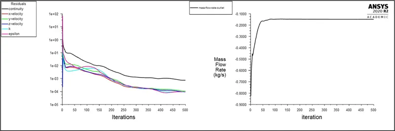
Fig. 8: Scaled Residuals and mass flow rate at the outlet plots for Baseline mesh using the Realisable k-`epsilon` turbulence model with SIMPLEC solver at 10% valve opening
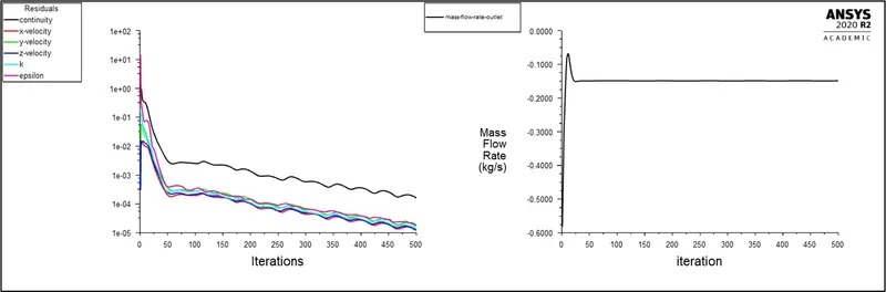
Fig. 9: Scaled Residuals and mass flow rate at the outlet plots for Baseline mesh using the Realisable k-`epsilon` turbulence model with COUPLED solver at 10% valve opening
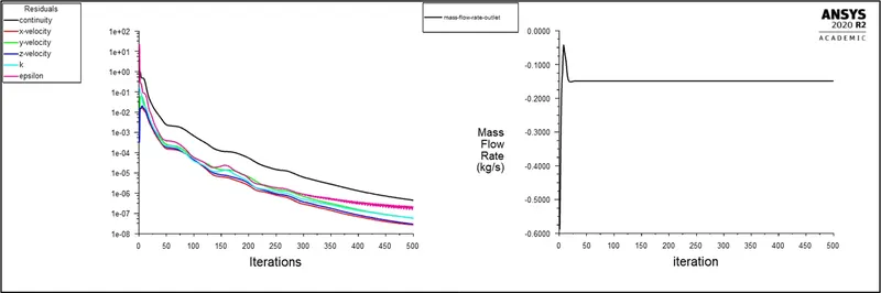
Fig. 10: Scaled Residuals and mass flow rate at the outlet plots for mesh 1 using the Realisable k-`epsilon` turbulence model with COUPLED solver at 10% valve opening
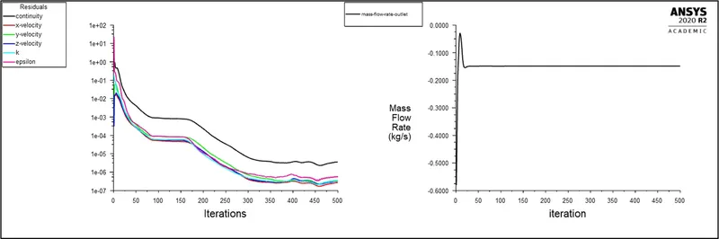
Fig. 11: Scaled Residuals and mass flow rate at the outlet plots for mesh 2 using the Realisable k-`epsilon` turbulence model with COUPLED solver at 10% valve opening
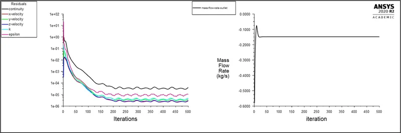
Fig. 12: Scaled Residuals and mass flow rate at the outlet plots for mesh 3 using the Realisable k-`epsilon` turbulence model with COUPLED solver at 10% valve opening
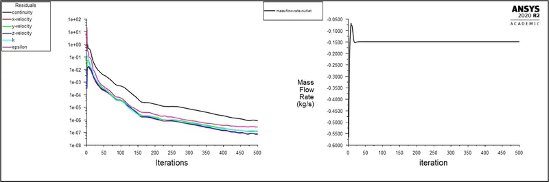
Fig. 13: Scaled Residuals and mass flow rate at the outlet plots for mesh 4 using the Realisable k-`epsilon` turbulence model with COUPLED solver at 10% valve opening
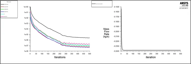
Fig. 14: Scaled Residuals and mass flow rate at the outlet plots for mesh 3 using the Realisable k-`epsilon` turbulence model with COUPLED solver at 20% valve opening
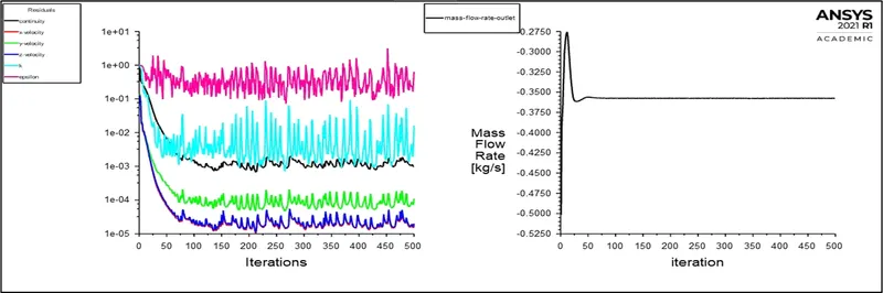
Fig. 15: Scaled Residuals and mass flow rate at the outlet plots for mesh 3 using the Realisable k-`epsilon` turbulence model with COUPLED solver at 30% valve opening
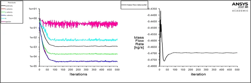
Fig. 16: Scaled Residuals and mass flow rate at the outlet plots for mesh 3 using the Realisable k-`epsilon` turbulence model with COUPLED solver at 40% valve opening
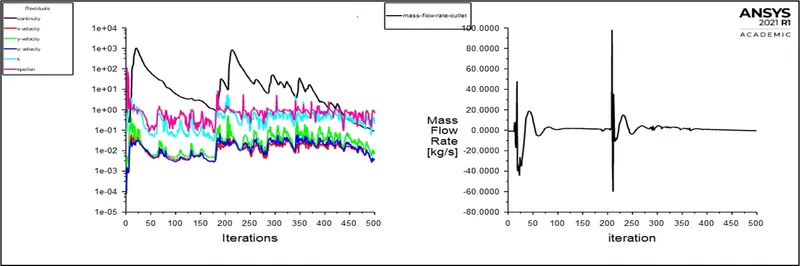
Fig. 17: Scaled Residuals and mass flow rate at the outlet plots for mesh 3 using the Realisable k-`epsilon` turbulence model with COUPLED solver at 50% valve opening
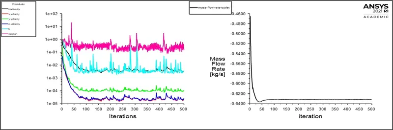
Fig. 18: Scaled Residuals and mass flow rate at the outlet plots for mesh 3 using the Realisable k-`epsilon` turbulence model with COUPLED solver at 60% valve opening
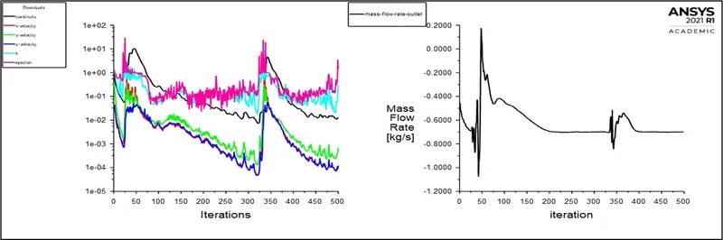
Fig. 19: Scaled Residuals and mass flow rate at the outlet plots for mesh 3 using the Realisable k-`epsilon` turbulence model with COUPLED solver at 70% valve opening
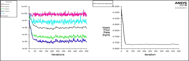
Fig. 20: Scaled Residuals and mass flow rate at the outlet plots for mesh 3 using the Realisable k-`epsilon` turbulence model with COUPLED solver at 80% valve opening
From Fig. 7, Fig. 8 and Fig. 9, it can be noticed that all three of the pressure-velocity coupling schemes have shown stable convergence with highly stable outputs as seen in the monitor plots well before they reach the total number of iterations indicating that a steady-state solution was obtained, however, the COUPLED scheme, as was also mentioned in Section 2.5.3 Mesh Refinement approach, has the lowest recorded residual limit values for almost all equations (except maybe for the continuity equation) while also taking the most computational time. This reconfirms the expected behaviour from each of the schemes. A similar trend in results is also observed from Fig. 10 to Fig. 13 in the simulation of different meshes with only the residuals expressing small and disproportionate amplitudes of oscillatory fluctuations and marginal differences in the numerical value output of the monitor plots. However, from Fig. 14 to Fig. 20, the residuals behave in an erratic manner as a consequence of different valve lift positions, also observed in the behaviour of the monitor plots in the case of 50% and 70% opening values although they largely represent stable values over the course of the specified iterations in the remaining cases.
3.Results
In Section 3.1, formulae to determine flow coefficient and flow factor are presented while in Section 3.1.1, velocity and static pressure gradient plots, streamlines and vector plots are highlighted along with tabulated information for mass flow rate at the outlet, and flow coefficient and flow factor values at different valve lift positions.
3.1 Evaluation of flow coefficient and flow factor
Flow coefficient can be described as a device's efficiency for permitting fluid flow, in this case of the gate valve, and can be determined based on the pressure drop across the device and the corresponding flow rate which is expressed mathematically as shown below:
`C_v = Q*sqrt((SG)/(Delta P)`; where (Eq. 2)
`Q` is rate of fluid flow (in US gallons/min),
`SG` represents specific gravity of fluid which equates to 1 for water, and
`Delta p` is the pressure drop across the valve (in psi), and
Flow factor is a similar quantity to the flow coefficient but the values for rate of fluid flow and pressure drop are instead expressed in the metric system i.e., `m^3/h` and bar respectively. The values of pressure drop for the given numerical problem are computed as the absolute difference between pressure values near the gate disc, as created using Expressions in Section 2.4 Post-Processing, to record the maximum possible variation at different intervals of lift. It should be noted though that the definitions of flow coefficient were based on flow of water at 60 oF for pressure drop of 1 lb/in^2 while of flow factor for temperature of water ranging between 5 - 30 oC and pressure drop of 1 bar. Alternatively, flow factor (`K_v`) can be expressed in relation to the flow coefficient as follows:
`K_v = 0.865*C_v` (Eq. 3)
| Quantity | Original Units | Converted Quantity | Converted Units | Value used for Conversion (Multiplied/Divided with respect to Original Units) |
| Mass Flow Rate | [kg s^-1] | Rate of fluid flow | (US gallons/min) | 21.44 (Multiplied) |
| Pressure Drop | (Pa) | Pressure Drop | (psi) | 0.000145038 (Multiplied) |
Table 19: Conversion Table for mass flow rate and pressure drop quantities for calculation of flow coefficient variable
3.1.1 Effect of different valve opening values
Fig. 21, Fig. 22, Fig. 23 and Fig. 24 shows the velocity and static pressure gradient plots along Plane 1 (defined in Section 2.4 Post-Processing), streamlines and vector plots to illustrate the variations in velocity and pressure values as well as the changing flow profiles near the gate disc. It can be seen that with increase in the valve opening from 10% to 80% relating to 10mm to 80mm lift values respectively, the velocity values increase and pressure values conversely decrease near the curvature region of the valve body and the beginning of outlet pipe regions especially in the case of 30mm and 40mm valve lift values before beginning to have a more even distribution across the length of the domain towards the exit point. This maybe attributed to the sudden rise in velocity of flow, relative to its initial lift position of 10mm, causing water to advance towards the low pressure region created in the curved area at a rapid rate. This behaviour of the fluid can also be observed in the streamlines and vector plots, especially after the gate disc, wherein the flow profiles undergo transition in its shape indicating the presence of a backflow region that decreases in intensity with the rise in valve lift values. Table 20 and Fig. 25 categorises data on mass flow rate at outlet, pressure drop, and corresponding flow coefficient and flow factor values at different valve lift positions and establishes a relation between the quantities indicating that for every rise in valve lift value by 10%, or an equivalent of 10mm, the flow coefficient and flow factor values also increase proportional to the amount of flow passing through the piping configuration and drop in pressure head across the valve interface. The significance of the flow coefficient and flow factor values is taken into consideration at the time of estimation and appropriate selection of the gate valve sizes by comparing against different manufacturers as it represents permissible flow capacities as well as corresponding effects on pressure of the given system.
For Mesh 3:
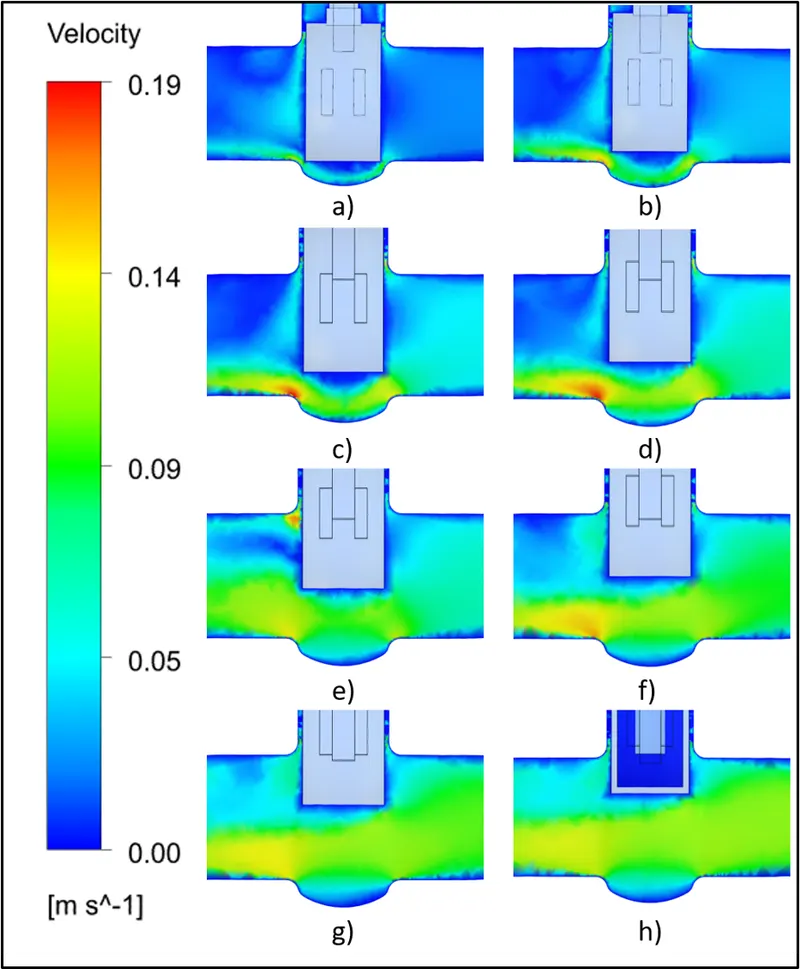
Fig. 21: Velocity contour plots along the mid plane (in YZ direction) for different valve lift values [a) 10mm, b) 20mm, c) 30mm, d) 40mm, e) 50mm, f) 60mm, g) 70mm, h) 80mm]
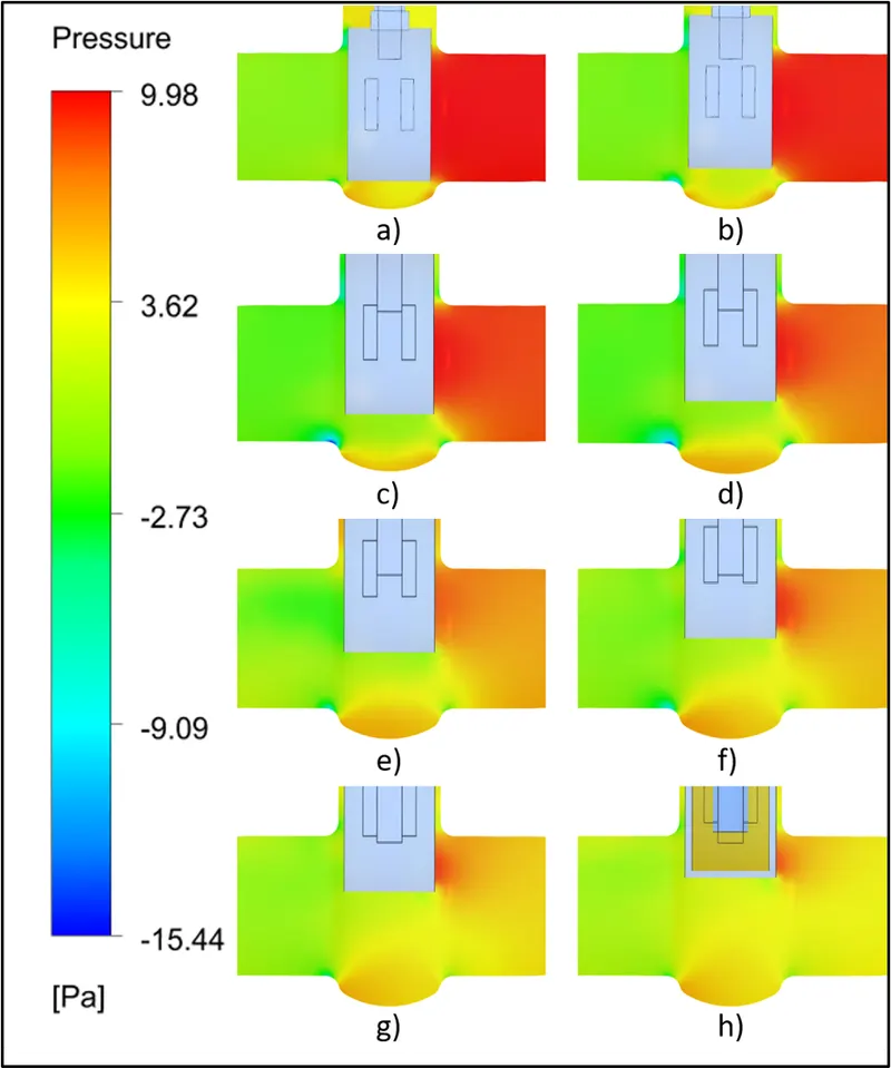
Fig. 22: Static pressure contour plots along the mid plane (in YZ direction) for different valve lift values [a) 10mm, b) 20mm, c) 30mm, d) 40mm, e) 50mm, f) 60mm, g) 70mm, h) 80mm]
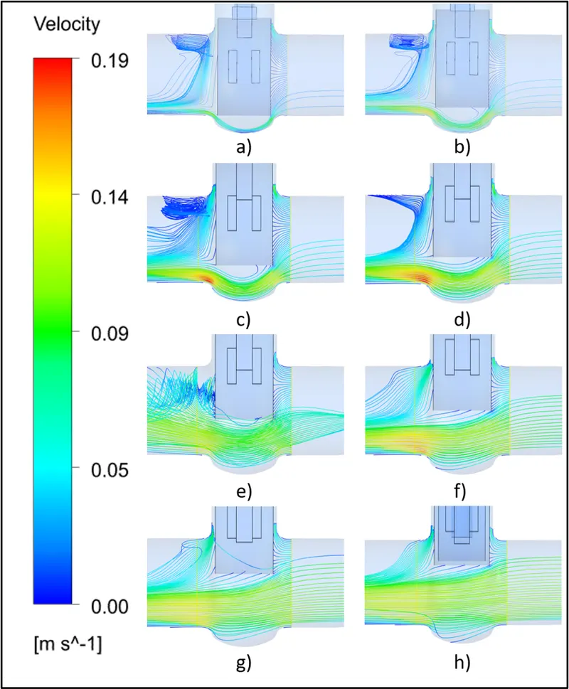
Fig. 23: Streamline plots along the mid plane (in YZ direction) for different valve lift values [a) 10mm, b) 20mm, c) 30mm, d) 40mm, e) 50mm, f) 60mm, g) 70mm, h) 80mm]
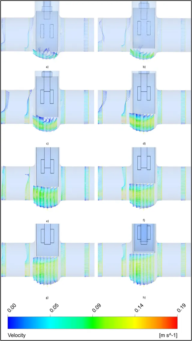
Fig. 24: Vector plots along the mid plane (in YZ direction) for different valve lift values [a) 10mm, b) 20mm, c) 30mm, d) 40mm, e) 50mm, f) 60mm, g) 70mm, h) 80mm]
|
Valve Opening (%) |
Valve Lift [m] |
Mass Flow Rate at outlet [kg s^-1] |
Pressure Drop (Pa) |
Flow coefficient (`C_v`) (Eq. 2 and Table 19) |
Flow factor (`K_v`) (Eq. 3) |
|
10 |
0.01 |
0.1487 |
10.1426 |
83.1228 |
71.9012 |
|
20 |
0.02 |
0.2383 |
10.3651 |
131.7714 |
113.9823 |
|
30 |
0.03 |
0.3576 |
10.1673 |
199.6542 |
172.7009 |
|
40 |
0.04 | 0.4695 | 9.3006 | 274.0716 | 237.0719 |
|
50 |
0.05 | 0.476 | 5.8676 | 349.8328 | 302.6054 |
|
60 |
0.06 | 0.6319 | 6.7069 | 434.3815 | 375.74 |
|
70 |
0.07 | 0.6989 | 4.9452 | 559.5089 | 483.9752 |
|
80 |
0.08 | 0.7649 | 3.0824 | 775.6111 | 670.9036 |
Table 20: Valve opening, valve lift, mass flow rate at the outlet, and flow coefficient and flow factor values for the given gate valve assembly model at constant input gauge total pressure of 10 Pascals
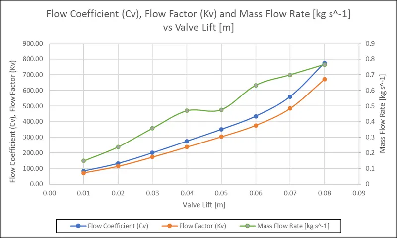
Fig. 25: Flow coefficient (`C_v`), flow factor (`K_v`), mass flow rate [kg s^-1] at the outlet values vs different positions of valve lift [m]
4. Discussion
Mass flow of water from the inlet to the outlet passage is controlled by the often manually operated handwheel of the gate valve which is rotated in either clockwise or anti-clockwise direction to linearly move the gate disc vertically downwards or upwards respectively. The amount of water as a function of time flowing across the gate disc interface during its vertical travel is typically non-linear, as also observed in Table 20 of Section 3 Results. The process of regulating flow at initial opening levels usually involves relatively high velocities that can lead to gradual wear and erosion of the gate and seats over its due course of operation combined with the induced vibrations leading to shortened service life of the valve. Flow coefficient and in turn the flow factor values of a valve, depending on the opening or valve lift values, represents the amount of fluid that can pass through it and the two quantities are directly proportional to each other implying that larger the opening in the valve, larger is the flow coefficient and flow factor values. The general approach adopted during selection of a gate valve size usually involves identifying the range of opening, based on the service conditions, and comparing the flow coefficient values between different valve sizes based on the curves representing the flow coefficient and/or flow factor values within the recognised range of opening to offer maximum benefits with regards to higher flow capacity and minimum pressure drop across the intended system.
5. Conclusion
The numerical analysis for the given gate valve model under steady state conditions for different valve opening positions, as a parametric study, using the Realisable k-`epsilon` turbulence model in ANSYS Fluent 2020 R2 and ANSYS Fluent 2021 R1 was well understood. The use of two different versions of ANSYS Fluent was undertaken due to unforeseen software issues on one of the two systems that faced difficulties in updating the solution during the parametric assessment. The relation between the values obtained at the outlet for mass flow rate at different valve lift settings provided a deeper insight into the development of velocity and pressure profiles. Additionally, the evaluation of flow coefficient and flow factor values for the different opening arrangements established the impact of governing flow and pressure conditions as well as its significance from the perspective of selection of gate valve sizes in different applications that aids in cost and maintenance benefits.