Week 3.5 - Deriving 4th order approximation of a 2nd order derivative using Taylor Table method

Aim : The objective is to derive a 4th order approximation of a 2nd order derivative using a Taylor Table method for approximation schemes of :

1. Central Differencing Scheme
2. Skewed right-sided scheme
3. Skewed light-sided scheme

Theory : Taylor Series formula is a representation of any function as an infinite sum of terms. These terms are calculated from the values of function’s derivatives at a single point.

With the help of the taylor series we calculated the forward,backward and central differencing for the first order of derivatives.

Forward differencing :

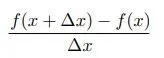
Backward Differencing :

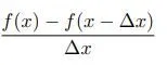
and similarly by combining different taylor series expansion we can come up with approximations of different orders like,

2nd order approximation for 2nd order of derivatives.

To calculate a lower order of approximations is easy as compared to the higher order like 3,4 or 5 order of approximations.So calculate for higher order of approximations there is an elegent way to do it known as Taylor Table.A Taylor Table is basically just collection of taylor series representation for each term for which we are expanding the taylor series.In Taylor Table the rows shows the terms of the Hypothesis Function with the unkown coefficients to find,and the coloumn consist of the commomn taylor series expansion terms for each terms of the row.

Requirements : Function for wich the solution has to be derived : f(x) = exp(x)*cos(x)

at x = `pi/3` dx = `(pi/40,pi/4000)` range of dx.

Second Derivative of the function : f''(x) = -2*exp(x)*cos(x) (in code is mentioned as analytical_derivative)

• To calculate the Number of Nodes for the central and the side skewed schemes.
• For symmetrical/centerd scheme: Number of Nodes(N) = Order of Derivative(P) + Order of Approximation(Q) - 1

N = 2 + 4 -1

N = 5 (Therefore we will need 5 nodes on the stencil to find the 4th order of approximation of the 2nd order of derivatives)

• For asymetric/skewed schemes : Number of Nodes(N) = Order of Derivative(P) + Order of Approximation(Q)

N = 2 + 4

N = 6

Now, we will derive the Taylor table for our challange:

• Right Sided Skewed : Here we will skeweing the values from the right side from the (i) point and as we calculated we need 6 nodes for the skewed scheme.

Hypothesis Function :

`dx^2 (d^2 u)/dx^2 = a*f(i)+b*f(i+1)+c*f(i+2)+d*f(i+3)+e*f(i+4)+g*f(i+5)`

we have to find the unknown coefficient to calculate the 2nd order derivative

	f(i)	f'(i)dx	f''(i)dx^2	f'''(i)dx^3	f''''(i)dx^4	f'''''(i)dx^5
af(i)	a	0	0	0	0	0
bf(i+1)	b	b	b/2	b/6	b/24	b/120
cf(i+2)	c	2c	4c/2	8c/6	16c/24	32c/120
df(i+3)	d	3d	9d/2	27d/6	81d/24	243d/120
ef(i+4)	e	4e	16e/2	67e/6	256e/24	1024e/120
gf(i+5)	g	5g	25g/2	125g/6	625g/24	3125g/120
sum_of_cofficients `approx (d^2u)/dx^2`	0	0	1	0	0	0

Here we only have 6 terms of the taylor series why because as there are only 6 nodes for required for calculating the 4th order approximation and also from the table we can see that we have only 6 unknown so we only need 6 terms to calculate those unknown too.If we add more terms we will only be over specifying the function thats all.

The 1 for the sum of the 3rd coloumn says that we only need that terms as it represents the second order derivative.

Writing all the coefficients together we will get

a+b+c+d+e+g = 0

b+2c+3d+4e+5g = 0

b/2+4c/2+9d/2+16e/2+25g/2 = 1

b/6+8c/6+27d/6+67e/6+125g/6 = 0

b/24+16c/24+81d/24+256e/24+625g/24 = 0

b/120+32c/120+243d/120+1024e/120+3125g/120 = 0

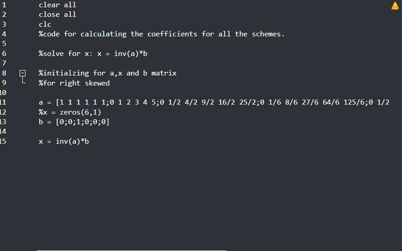
linear equation obtained from above equation is written in matrix form and are solved by matrix inversion method

A*X = B

X = inv(A)*B

where,A = `[[1,1,1,1,1,1], [0,1,2,3,4,5],[0,1/2,4/2,9/2,16/2,25/2],[0,1/6,8/6,27/6,64/6,125/6],[0,1/24,16/24,81/24,256/24,625/24],[0,1/120,32/120,243/120,1024/120,3125/120]]`

X = `((a),(b),(c),(d),(e),(g))`

B = `((0),(0),(1),(0),(0),(0))`

plugging these values in Matlab and calculate the unknown values as shown below

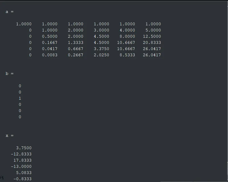
From the code: a = 3.7500

b = -12.8333

c = 17.8333

d = -13.0000

e = 5.0833

g = -0.8333

Writting the Hypothesis Function with the values obtained

`(d^2u)/dx^2 approx ( (3.7500)*f(i)+(-12.833)*f(i+1)+(17.8333)*f(i+2)+(-13.0000)*f(i+3)+(5.0833)*f(i+4)+(-0.8333)*f(i+5))/(dx^2)`

• Left Sided Skewed :

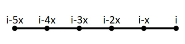
Hypothesis Function :

`dx^2 (d^2 u)/dx^2 = a*f(i-5)+b*f(i-4)+c*f(i-3)+d*f(i-2)+e*f(i-1)+g*f(i)`

Taylor table

	f(i)	f'(i)dx	f''(i)dx^2	f'''(i)dx^3	f''''(i)dx^4	f'''''(i)dx^5
af(i-5)	a	-5a	25a/2	-125a/6	625a/24	-3125a/120
bf(i-4)	b	-4b	16b/2	-64b/6	256b/24	-1024b/120
cf(i-3)	c	-3c	9c/2	-27c/6	81c/24	-248c/120
df(i-2)	d	-2d	4d/2	8d/6	16d/24	32d/120
ef(i-1)	e	-1e	e/2	e/6	e/24	e/120
gf(i)	g	0	0	0	0	0
sum of coefficients	0	0	1	0	0	0

Now,similarly we will create the matrix and solve for the unknowns.

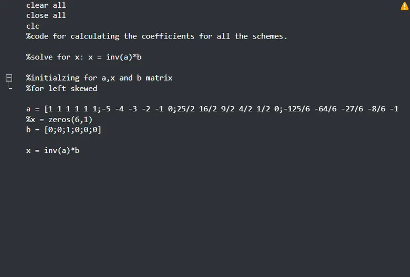
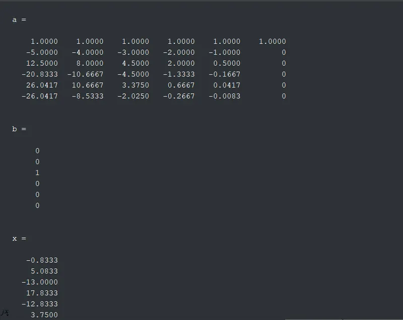
a = -0.8333

b = 5.0833

c = -13.0000

d = 17.8333

e = -12.8333

g = 3.7500

wrting the hypothesis function with the coefficient values

`(d^2 u)/dx^2 approx ((-0.8333)*f(i-5)+(5.0833)*f(i-4)+(-13.0000)*f(i-3)+(17.8333)*f(i-2)+(-12.8333)*f(i-1)+(3.7500)*f(i))/(dx^2)`

• Centered Difference Scheme :

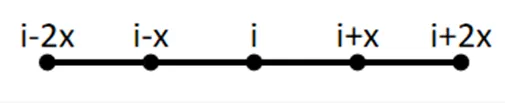
Hypothesis Function :

`dx^2 (d^2 u)/dx^2 = a*f(i-2)+b*f(i-1)+c*f(i)+d*f(i+1)+e*f(i+2)`

Taylor Table :

	f(i)	f'(i)dx	f''(i)dx^2	f'''(i)dx^3	f''''(i)dx^4
af(i-2)	a	-2a	4a/2	-8a/6	16a/24
bf(i-1)	b	-b	b/2	-b/6	b/24
cf(i)	c	0	0	0	0
df(i+1)	d	d	d/2	d/6	d/24
ef(i+2)	e	2e	4e/2	8e/6	16e/24
sum of coefficients	0	0	1	0	0

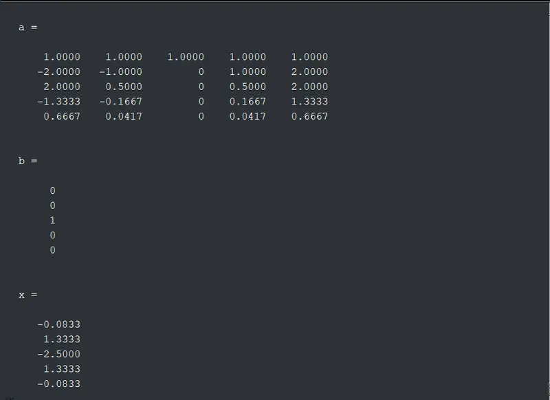
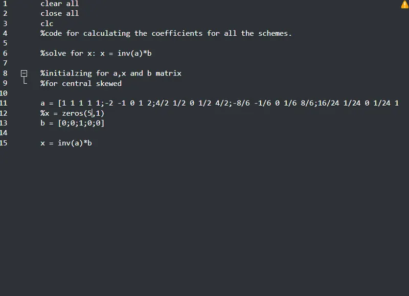
a = -0.0833

b = 1.3333

c = -2.5000

d = 1.3333

e = -0.0833

wrting the hypothesis function with the coefficient values

`(d^2 u)/dx^2 approx ((-0.0833)*f(i-2)+(1.3333)*f(i-1)+(-2.5000)*f(i)+(1.3333)*f(i+1)+(-0.0833)*f(i+2))/(dx^2)`

• To prove that our approximation is 4th order approximation :

For symmetrical/centerd scheme: Order of Approximation(Q) = Number of Nodes(N) - Order of Derivative(P) + 1

Q = 5 - 2 + 1

Q = 4

For asymetric/skewed schemes : Order of Approximation(Q)= Number of Nodes(N) - Order of Derivative(P)

Q = 6 - 2

Q = 4

• Matlab Code:
• Code for the function of second order scheme:

%function code for the center scheme difference

function central_scheme_error = Center(x,dx);

%analytical derivative f''(x) = -2*exp(x)*sin(x)
analytical_derivative = -2*exp(x)*sin(x);

%initialzing the coefficients values
a =-0.0833;
b = 1.3333;
c = -2.5000;
d = 1.3333;
e = -0.0833;

%central_diff_scheme= (af(x-2dx)+bf(x-dx)+cf(x)+df(x+dx)+ef(x+2dx))/dx^2
central_diff_scheme = (a*(exp(x-2*dx)*cos(x-2*dx))+b*(exp(x-dx)*cos(x-dx))+c*(exp(x)*cos(x))+d*(exp(x+dx)*cos(x+dx))+e*(exp(x+2*dx)*cos(x+2*dx)))/(dx^2);

%difference between the analytical and numerical solution

central_scheme_error = abs(central_diff_scheme - analytical_derivative);
end

• Code for Right skewed scheme :

%function code for right skewed scheme 

function right_scheme_error = Right(x,dx);

%analytical derivative f''(x) = -2*exp(x)*sin(x)
analytical_derivative = -2*exp(x)*sin(x);

%initialzing the coefficients values
a = 3.7500;
b = -12.8333;
c = 17.8333;
d = -13.0000;
e = 5.0833;
g = -0.8333;

%right_diff_scheme= (af(x)+bf(x+dx)+cf(x+2dx)+df(x+3dx)+ef(x+4dx)+gf(x+5dx))/dx^2
right_diff_scheme = (a*(exp(x)*cos(x))+b*(exp(x+dx)*cos(x+dx))+c*(exp(x+2*dx)*cos(x+2*dx))+d*(exp(x+3*dx)*cos(x+3*dx))+e*(exp(x+4*dx)*cos(x+4*dx))+g*(exp(x+5*dx)*cos(x+5*dx)))/(dx^2);

%difference between the analytical and numerical solution

right_scheme_error = abs(right_diff_scheme - analytical_derivative);
end

• Code for left skewed scheme :

%function code for left skewed scheme 

function left_scheme_error = Left(x,dx);

%analytical derivative f''(x) = -2*exp(x)*sin(x)
analytical_derivative = -2*exp(x)*sin(x);

%initialzing the coefficients values
a = -0.8333;
b = 5.0833;
c = -13.000;
d = 17.8333;
e = -12.8333;
g = 3.7500;

%left_diff_scheme= (af(x-5dx)+bf(x-4dx)+cf(x-3dx)+df(x-2dx)+ef(x-dx)+gf(x))/dx^2
left_diff_scheme = (a*(exp(x-5*dx)*cos(x-5*dx))+b*(exp(x-4*dx)*cos(x-4*dx))+c*(exp(x-3*dx)*cos(x-3*dx))+d*(exp(x-2*dx)*cos(x-2*dx))+e*(exp(x-dx)*cos(x-dx))+g*(exp(x)*cos(x)))/(dx^2);

%difference between the analytical and numerical solution

left_scheme_error = abs(left_diff_scheme - analytical_derivative);
end

• Main code :

clear all
close all
clc
%main code for calculating the error over range of dx
%initializing the x and dx values
x = pi/3;
dx = linspace(pi/40,pi/40000,20);
%calculating the error over range of dx
for i = 1:length(dx)
RS_error(i) = Right(x,dx(i));
LS_error(i) = Left(x,dx(i));
CS_error(i) = Center(x,dx(i));
end
%plotting graph for dx v/s schemes
figure(1);
plot(dx,CS_error,'Color','r','LineStyle','-','LineWidth',0.8);
xlabel('Range of dx');
ylabel('Schemes Error');
hold on;
plot(dx,RS_error,'Color','b','LineStyle','--','LineWidth',0.8,'Marker','o');
hold on;
plot(dx,LS_error,'Color','m','LineStyle',':','LineWidth',0.8);
title('Range(dx) v/s Schemes');
legend(': Central Scheme',': Right Scheme',': Left Scheme');
grid on;
figure(2);
loglog(dx,CS_error,'Color','r','LineStyle','-','LineWidth',1.2);
xlabel('Range of dx');
ylabel('Schemes Error');
hold on;
loglog(dx,RS_error,'Color','b','LineStyle','--','LineWidth',1.2);
hold on;
loglog(dx,LS_error,'Color','m','LineStyle',':','LineWidth',1.2);
title('Log Plot:Range(dx) v/s Schemes');
legend(': Central Scheme',': Right Scheme',': Left Scheme');
grid on;

• we have created the three function code for each schemes and the coefficiencts values are initialized in each code rescpectively.the analytical derivative is also derived for each value of dx.the output of the function codes is the error values between the numerical scheme and the exact or analytical solution.
• Similarly to previous challange we discretized the solution for each scheme for the range of dx values.To execute the code properly we used the 'for' loop for executing the functions written for each scheme over the range of dx.
• In the main code the values of the function are stored in the RS_error,LS_error and CS_error which are right scheme,left scheme and center sceheme error
• And finally the plots are drawn in the log graph which is better as the error values increases drastically with increase in dx value.

Result :

log plot for range of dx v/s the schemes

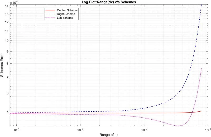
from the plot we can conclude that the error value for the Second Order Scheme is very less as compared to the Right and Left Skewed Schemes.That is because for the centered order schemes the values for the derivative is calculated by considering the nodes from both side and that provides a good accuracy than the skewed schemes which just takes the values from only one side of the considered node.

Why a Skewed Schemes is useful ?

When the system does'nt contain much information on both sides of the interest point .In such cases only skewed schemes are useful as they only required the information from the one side of the nodes.

What can a Skewed Scheme can do that a Center Scheme cannot do ?

CDS cannot be employed at the boundary nodes due to unavailability of right and left nodes at the same time.In such cases the skewed scheme will be much useful.