Week 11 - Simulation of Flow through a pipe in OpenFoam
Aim : To simulate an incompressible,laminar,Newtonian axi - symmetric fluid through a pipe.Apply the Wedge boundary condition to the geometry and automate a fully functional blockMeshDict file.Compare the numerical result with the analytical profile.
Expected Results
- Validate Hydro-dynamic length with the numerical result
- Validate the fully developed flow velocity profile with its analytical profile
- Validate maximum velocity and pressured drop for fully developed flow
- Post-process Shear stress and validate wall shear stress for fully developed flow
Theory :
Liquid and gas flow through pipes or ducts is commonly used in heating and cooling applications and fluid distribution networks.The fluid in such applications is usually forced to flow by a fan or pumpthrough a flow section.The friction that is caused by shear stress is directly related to prerssure drop and head loss during flow through pipe and ducts.The pressure drop is then used to determine the pumping power requirement. A typical piping system involves pipes of different diameters connected to each other by various fitting or elbows to route the fluid,valve to control the flow rate and pumps to pressurize the fluid.Therefore,problems and simulation for fluid through pipe are very important engineering problems to solve.
- Pipes with circular cross-sections are used to regulate fluids as they can handle very large pressure difference without undergoing significant distortion.
The fluid velocity in a pipe changes from zero at the surface because of no-slip(flow velocity at the wall becomes zero) condition to a maximum at the pipe centre.
The average velocity is the velocity that remains constant in incompressible flow when the cross-section of the pipe is constant.
- due to no-slip condition fluid at the wall completely stops.
- this slows down adjacent layers of the fluid,that results in friction between the fluid layers.
- to make up for this reduction and keep the mass flow inside the pipe constant,velocity increses at centre of the pipe,resulting in Velocity gradient along the pipe.
- The region of the flow in which the effects of the viscous shearing forces caused by fluid viscosity are felt is called the boundary layer.
- The thickness of this boundary layer increases in the flow direction untill the boundary layer reaches the pipe centre and thus fills the entire pipe.
- The region from inlet of the pipe to the point at which the boundary layer merges with the centerline is called Hydrodynamic Entrance Region,and the lenght of this region is called Hydrodynamic Entrance Length (`L_h`).
- Flow in this region is called Hydrodynamically Developing Flow as the velocity profile develops here.
- Further downstream from this region is called Hydrodynamically Fully Developed region.Here the velocity profile develops fully and takes the shape of Parabola in laminar flow.
- Hagen-Poiseuilles Theory :The Hagen-Poiseuille equation describes the flow of a viscous fluid through a cylindrical pipe or tube under laminar flow conditions. It is based on a number of assumptions, including that the fluid is incompressible, the flow is steady, and the fluid velocity profile is parabolic.The Hagen-Poiseuille equation provides a fundamental understanding of fluid flow in pipes and is widely used in various fields, including engineering, physics, and biology, to analyze and predict fluid flow rates in different systems. A Pressure Drop due to viscous effects represent and irreversible Pressure Loss.It is called Pressure Loss to emphasize a loss just like head loss.
Hagen-Poiseuilles equation : `Delta p = (8muV_(avg)L)/R^4=(32muV_(avg)L)/D^2`
where `mu` = dynamic viscosity , D = diameter of the pipe, L = lenght of the pipe.
From the given equation we can say that pressure loss is directly proportional to viscosity of the fluid and the lenght of the pipe but is also inversely proportional to the quadraple of radius.Emphasizing on the radius,The smaller the radius the the smaller will be the flow rate while the larger flow rate need a large diameter.In case of the pressure loss we can increase the power requirement of the pump by reducing th diameter of the pipe and vice-versa.
Note : This equation does not hold close to the pipe entrance as there is no changes in the fluid.
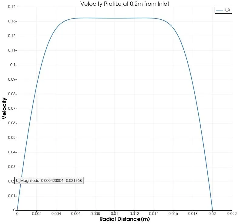
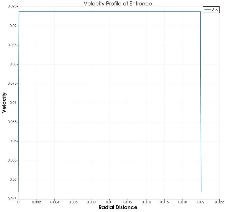 This image shows the velocity profile at the entrance of the pipe which can be seen perfectly stable undisturbed rectangle rather than an parabola from fully developed region.The above statement holds true for the flow at the entrance equations does not hold good.
The equation also fails for low viscosity,wide and/or short pipes.Low viscosity or a wide pipe may result in turbulent flow, making it necessary to use more complex models, such as Darcy-Weisbach equation.
The ratio of length to radius of a pipe should be greater than one forty-eighth of the Reynolds Number for the Hagen–Poiseuille law to be valid.When the length-to-radius ratio is smaller than this threshold, the flow is more likely to be affected by factors such as pipe entrance effects, flow disturbances, or incomplete development of velocity profile. In such cases, the Hagen-Poiseuille law may not accurately describe the flow behavior.For our case this ratio satisfies the condition and the simulation runs perfectly.
Calcualtions :
- For this project the fluid is considered as water at constant Temperature of 25 C.
`rho = 997.13 (kg)/m^3`
`mu = 0.89e^(-3) (kg)/(m*s)`
Reynolds Number (Re) = 2100
D = 0.02 m (Diameter of circle)
- Average Velocity(`V_(avg)`) : `V_(avg) = (Re * mu)/(rho* D)`
`V_(avg) = 0.093 m/s`
- Maximum Velocity(`U_max`) : `U_(max) = 2*V_(avg) = 0.186 m/s`
- Entrane Lenght (`L_h`) : `L_h = 0.66*Re*D = 2.52 m`
- Total lenght of pipe : `L approx 3 m` (To let the flow fully develop).
- Pressure Drop (`Deltap`) : `Deltap = (32muV_(avg)L)/(D^2)`= 19.887 Pa
Procedure :
- Copy the Tuturial from tutorial package of openfoam in the run folder by following this command : cp -r cavity $FOAM_RUN/test_04.
- We also have to write a fully functional blockMeshDict file in Matlab or Octave and then use that for our copied case file.
- Calculate all other properties that requires change for our case.Like value for Inlet velocity,pressure value and time step values.
- Run the simulation for 25sec and post-process the result in Paraview.
- blockMeshDict file parse code :-
clear all
close all
clc

%Inputs important for mesh file
D = 0.02;              %Diameter of Pipe in m
R = D/2;               %Radius of the pipe
theta = 4;             %Angle of the Wedge
L = 3;                 %Total lenght of Pipe in m

%Header Context
h1 = '/*--------------------------------*- C++ -*----------------------------------*\';
h2 = '  =========                 | ';
h3 = '  \\      /  F ield         | OpenFOAM: The Open Source CFD Toolbox';
h4 = '   \\    /   O peration     | Website:  https://openfoam.org';
h5 = '    \\  /    A nd           | Version:  10';
h6 = '     \\/     M anipulation  |  ';
h7 = '\*---------------------------------------------------------------------------*/';
h8 = 'FoamFile  ';

%Dictionary Context
d1 = '{  ';
d2 = '    format      ascii; ';
d3 = '    class       dictionary;  ';
d4 = '    object      blockMeshDict;  ';
d5 = '}';
d6 = '// * * * * * * * * * * * * * * * * * * * * * * * * * * * * * * * * * * * * * // ';

%ConversionToMeters
conv = 'convertToMeters 1;';

%Initializing vertices
v0 = [0 0 0];
v1 = [0 R*cosd(theta/2) R*sind(theta/2)];
v2 = [0 R*cosd(theta/2) -R*sind(theta/2)];
v3 = [L 0 0];
v4 = [L R*cosd(theta/2) R*sind(theta/2)];
v5 = [L R*cosd(theta/2) -R*sind(theta/2)];

%Initializing arcs
arc1 = [0 R 0];
arc2 = [L R 0];

%Naming the file and writting the context
b = fopen('blockMeshDict.txt','w')

fprintf(b,'%s\n',h1);
fprintf(b,'%s\n',h2);
fprintf(b,'%s\n',h3);
fprintf(b,'%s\n',h4);
fprintf(b,'%s\n',h5);
fprintf(b,'%s\n',h6);
fprintf(b,'%s\n',h7);
fprintf(b,'%s\n',h8);

fprintf(b,'%s\n',d1);
##fprintf(b,'%s\n',d);
fprintf(b,'%s\n',d2);
fprintf(b,'%s\n',d3);
fprintf(b,'%s\n',d4);
fprintf(b,'%s\n',d5);
fprintf(b,'%s\n',d6);

fprintf(b,'\n');

fprintf(b,'%s\n',conv);

%Writing Vertices
fprintf(b,'\n');
fprintf(b,'%s\n','vertices');
fprintf(b,'%s\n','(');
fprintf(b,'\t(%f %f %f)\n',v0(1),v0(2),v0(3));
fprintf(b,'\t(%f %f %f)\n',v1(1),v1(2),v1(3));
fprintf(b,'\t(%f %f %f)\n',v2(1),v2(2),v2(3));
fprintf(b,'\t(%f %f %f)\n',v3(1),v3(2),v3(3));
fprintf(b,'\t(%f %f %f)\n',v4(1),v4(2),v4(3));
fprintf(b,'\t(%f %f %f)\n',v5(1),v5(2),v5(3));
fprintf(b,'%s\n',');');

%Writing Block
fprintf(b,'%s\n',' ');
fprintf(b,'%s\n','blocks');
fprintf(b,'%s\n','(');
fprintf(b,'\t%s\n','hex (0 2 1 0 3 5 4 3) (30 1 300) simpleGrading (1 1 1)')
fprintf(b,');\n');

%Writing Edges
fprintf(b,'%s\n',' ');
fprintf(b,'%s\n','edges');
fprintf(b,'%s\n','(');
fprintf(b,'\t arc 1 2 (%f %f %f)\n',arc1(1),arc1(2),arc1(3));
fprintf(b,'\t arc 5 4 (%f %f %f)\n',arc2(1),arc2(2),arc2(3));
fprintf(b,');\n');


%Writing Boundaries
fprintf(b,'%s\n',' ');
fprintf(b,'%s\n','boundary');
fprintf(b,'%s\n','(');

%Inlet Boundary
fprintf(b,'\t%s\n','Inlet');
fprintf(b,'\t%s\n','{');
fprintf(b,'\t\t%s\n','type patch;');
fprintf(b,'\t\t%s\n','faces');
fprintf(b,'\t\t%s\n','(');
fprintf(b,'\t\t\t%s\n','(0 1 2 0)');
fprintf(b,'\t\t%s\n',');');
fprintf(b,'\t%s\n','}');

%Outlet Wall
fprintf(b,'\t%s\n','Outlet');
fprintf(b,'\t%s\n','{');
fprintf(b,'\t\t%s\n','type patch;');
fprintf(b,'\t\t%s\n','faces');
fprintf(b,'\t\t%s\n','(');
fprintf(b,'\t\t\t%s\n','(3 5 4 3)');
fprintf(b,'\t\t%s\n',');');
fprintf(b,'\t%s\n','}');

%Axis
fprintf(b,'\t%s\n','Axis');
fprintf(b,'\t%s\n','{');
fprintf(b,'\t\t%s\n','type empty;');
fprintf(b,'\t\t%s\n','faces');
fprintf(b,'\t\t%s\n','(');
fprintf(b,'\t\t\t%s\n','(3 0 0 3)');
fprintf(b,'\t\t%s\n',');');
fprintf(b,'\t%s\n','}');

%Front_Wedge
fprintf(b,'\t%s\n','Front_wedge');
fprintf(b,'\t%s\n','{');
fprintf(b,'\t\t%s\n','type wedge;');
fprintf(b,'\t\t%s\n','faces');
fprintf(b,'\t\t%s\n','(');
fprintf(b,'\t\t\t%s\n','(0 3 4 1)');
fprintf(b,'\t\t%s\n',');');
fprintf(b,'\t%s\n','}');

%Back_wedge
fprintf(b,'\t%s\n','Back_wedge');
fprintf(b,'\t%s\n','{');
fprintf(b,'\t\t%s\n','type wedge;');
fprintf(b,'\t\t%s\n','faces');
fprintf(b,'\t\t%s\n','(');
fprintf(b,'\t\t\t%s\n','(5 3 0 2)');
fprintf(b,'\t\t%s\n',');');
fprintf(b,'\t%s\n','}');

%Wall
fprintf(b,'\t%s\n','Wall');
fprintf(b,'\t%s\n','{');
fprintf(b,'\t\t%s\n','type wall;');
fprintf(b,'\t\t%s\n','faces');
fprintf(b,'\t\t%s\n','(');
fprintf(b,'\t\t\t%s\n','(1 4 5 2)');
fprintf(b,'\t\t%s\n',');');
fprintf(b,'\t%s\n','}');

fprintf(b,'%s\n',');');

%Merging Patch Pairs
fprintf(b,'%s\n',' ');
fprintf(b,'%s\n','mergePatchPairs');
fprintf(b,'%s\n','(');
fprintf(b,'%s\n',');');
fprintf(b,'\n');
fprintf(b,'// ************************************************************************* //\n');

fclose(b);
/*--------------------------------*- C++ -*----------------------------------*\
  =========                 |
  \\      /  F ield         | OpenFOAM: The Open Source CFD Toolbox
   \\    /   O peration     | Website:  https://openfoam.org
    \\  /    A nd           | Version:  10
     \\/     M anipulation  |
\*---------------------------------------------------------------------------*/
FoamFile
{
    format      ascii;
    class       dictionary;
    object      blockMeshDict;
}
// * * * * * * * * * * * * * * * * * * * * * * * * * * * * * * * * * * * * * //

convertToMeters 1;

vertices
(
	(0.000000 0.000000 0.000000)
	(0.000000 0.009994 0.000349)
	(0.000000 0.009994 -0.000349)
	(3.000000 0.000000 0.000000)
	(3.000000 0.009994 0.000349)
	(3.000000 0.009994 -0.000349)
);

blocks
(
	hex (0 2 1 0 3 5 4 3) (50 1 500) simpleGrading (0.2000 1 1)
);

edges
(
	 arc 1 2 (0.000000 0.010000 0.000000)
	 arc 5 4 (3.000000 0.010000 0.000000)
);

boundary
(
	Inlet
	{
		type patch;
		faces
		(
			(0 1 2 0)
		);
	}
	Outlet
	{
		type patch;
		faces
		(
			(3 5 4 3)
		);
	}
	Axis
	{
		type empty;
		faces
		(
			(3 0 0 3)
		);
	}
	Front_wedge
	{
		type wedge;
		faces
		(
			(0 3 4 1)
		);
	}
	Back_wedge
	{
		type wedge;
		faces
		(
			(5 3 0 2)
		);
	}
	Wall
	{
		type wall;
		faces
		(
			(1 4 5 2)
		);
	}
);

mergePatchPairs
(
);

// ************************************************************************* //
Explanation : blockMeshDict file is very formatted and each and every line has to be used to write a fully functional file to run.
each and every line of header part and dictionary part are stored in the variable.All the vertices are also initialized before writting them the file.
Now to write the file first we will open the file and to write into it we will pass the command 'r' that is shown in the code.Printing all the important parts of the file and then closing the file.
This file is then copied in the blockMeshDict file in the copied test file that will be executed.
Also changing the values of the velocity field as well as the pressure field in the 0 file folder.
- p file :- The icoFoam solver uses the pressure value as kinematic pressure that is defined as the ratio of pressure drop to density of the fluid.
`p_k = (Deltap)/rho (m^2)/s^2`
/*--------------------------------*- C++ -*----------------------------------*\
  =========                 |
  \\      /  F ield         | OpenFOAM: The Open Source CFD Toolbox
   \\    /   O peration     | Website:  https://openfoam.org
    \\  /    A nd           | Version:  10
     \\/     M anipulation  |
\*---------------------------------------------------------------------------*/
FoamFile
{
    format      ascii;
    class       volScalarField;
    object      p;
}
// * * * * * * * * * * * * * * * * * * * * * * * * * * * * * * * * * * * * * //

dimensions      [0 2 -2 0 0 0 0];

internalField   uniform 0;

boundaryField
{
    Inlet
    {
        type            zeroGradient;
    }
    Outlet
    {
        type            fixedValue;
        value           uniform 0.020081227;
    }
    Axis
    {
        type            empty;
    }
    Front_wedge
    {
        type            wedge;
    }
    Back_wedge
    {
        type            wedge;
    }
    Wall
    {
        type            zeroGradient;
    }
}

// ************************************************************************* //
- U file :- The velocity of the fluid is calculated by the reynolds number formula and the value is initialise in positive x-direction.
/*--------------------------------*- C++ -*----------------------------------*\
  =========                 |
  \\      /  F ield         | OpenFOAM: The Open Source CFD Toolbox
   \\    /   O peration     | Website:  https://openfoam.org
    \\  /    A nd           | Version:  10
     \\/     M anipulation  |
\*---------------------------------------------------------------------------*/
FoamFile
{
    format      ascii;
    class       volVectorField;
    object      U;
}
// * * * * * * * * * * * * * * * * * * * * * * * * * * * * * * * * * * * * * //

dimensions      [0 1 -1 0 0 0 0];

internalField   uniform (0 0 0);

boundaryField
{
    Inlet
    {
        type            fixedValue;
        value           uniform (0.0937312 0 0);
    }
    Outlet
    {
        type            zeroGradient;
    }
    Axis
    {
        type            empty;
    }
    Front_wedge
    {
        type            wedge;
    }
    Back_wedge
    {
        type            wedge;
    }
    Wall
    {
        type            fixedValue;
        value           uniform (0 0 0);
    }
}

// ************************************************************************* //
For the top wall of the pipe we have initilized a no-slip boundary condition.
- controlDict file :- The simulation is ran for 25sec and the dt value is calculated to keep the Courant Number less than 1,dt value is calculated by the formula
`dt = (CFL*dx)/(v_(avg)`
/*--------------------------------*- C++ -*----------------------------------*\
  =========                 |
  \\      /  F ield         | OpenFOAM: The Open Source CFD Toolbox
   \\    /   O peration     | Website:  https://openfoam.org
    \\  /    A nd           | Version:  10
     \\/     M anipulation  |
\*---------------------------------------------------------------------------*/
FoamFile
{
    format      ascii;
    class       dictionary;
    location    "system";
    object      controlDict;
}
// * * * * * * * * * * * * * * * * * * * * * * * * * * * * * * * * * * * * * //

application     icoFoam;

startFrom       startTime;

startTime       0;

stopAt          endTime;

endTime         25;

deltaT          0.01;

writeControl    timeStep;

writeInterval   20;

purgeWrite      0;

writeFormat     ascii;

writePrecision  6;

writeCompression off;

timeFormat      general;

timePrecision   6;

runTimeModifiable true;


// ************************************************************************* //
- physicalProperties :- this is located in the constant folder and this contains the kinematic viscositu value that can be calculated by the formula `nu = mu/rho`
/*--------------------------------*- C++ -*----------------------------------*\
  =========                 |
  \\      /  F ield         | OpenFOAM: The Open Source CFD Toolbox
   \\    /   O peration     | Website:  https://openfoam.org
    \\  /    A nd           | Version:  10
     \\/     M anipulation  |
\*---------------------------------------------------------------------------*/
FoamFile
{
    format      ascii;
    class       dictionary;
    location    "constant";
    object      physicalProperties;
}
// * * * * * * * * * * * * * * * * * * * * * * * * * * * * * * * * * * * * * //

nu              [0 2 -1 0 0 0 0] 0.892678e-6;


// ************************************************************************* //
Results :-
Mesh
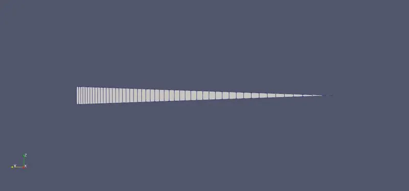
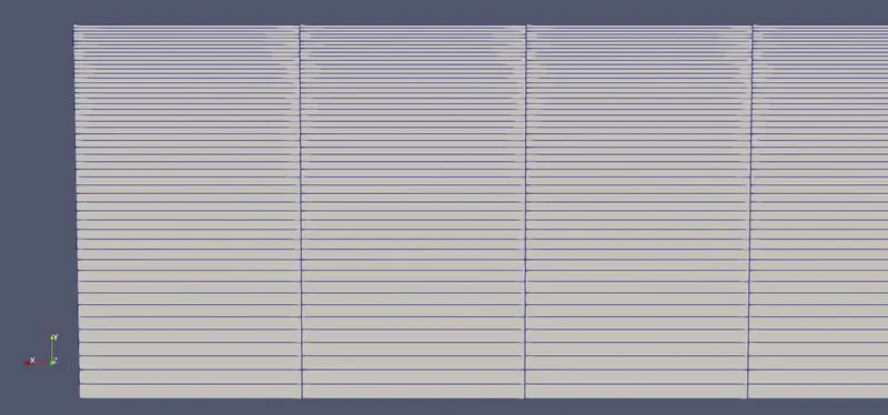
Velocity at Inlet
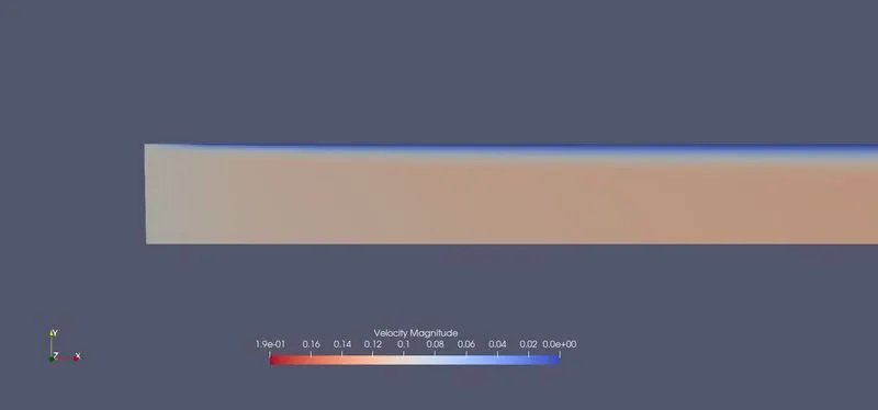
Velocity at Mid-Section
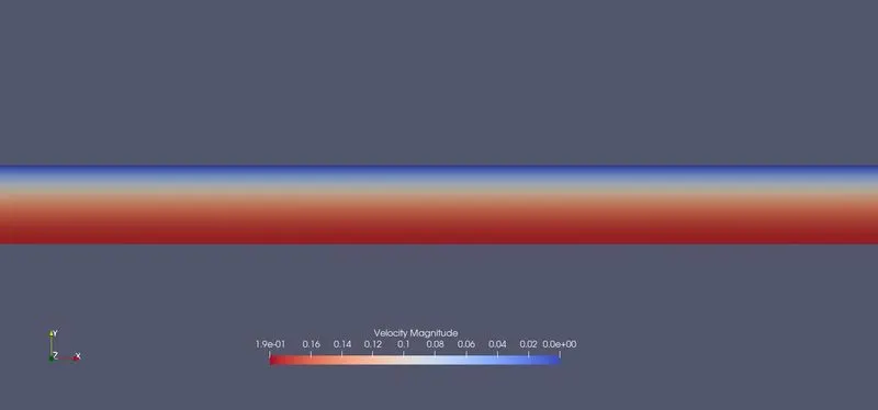
Velocity at Outlet
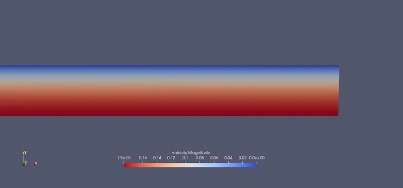
Mirroring results in Paraview :
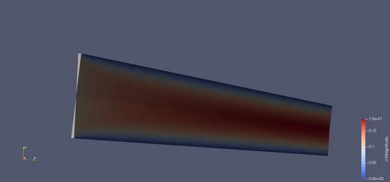
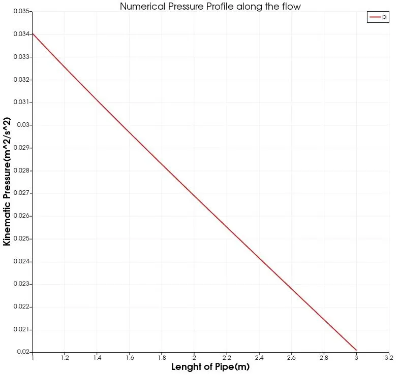
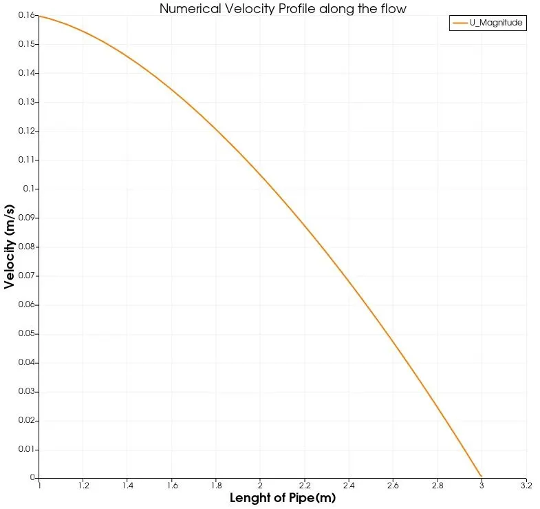
Velocity and Pressure Profile along the flow :
Pressure Profile
Velocity Profile
Velocity Profiles at different section in Radial Direction :
Velocity Profile at Hydrodynamically Entrance Region :
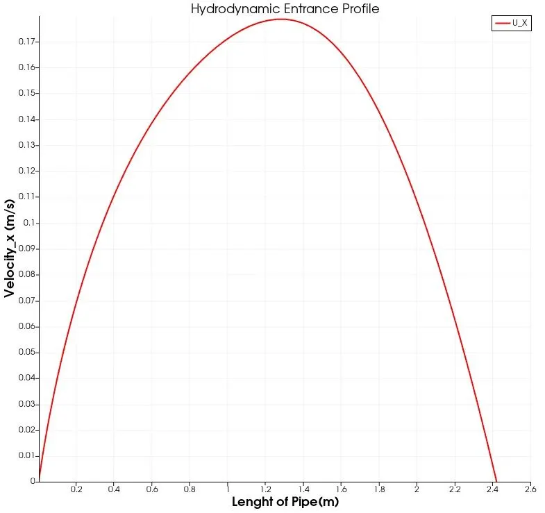 the simulated hydrodynamic entrance region validates the analytical hydrodynamic lenght.
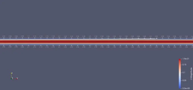 In laminar flow the viscosity of fluid,shape of the pipe and velocity influence the development of the flow,as the flow go further downstream the flow fully developes and become constant.The point where the flow fully develops and reaches consistent profile is called as Hydrocdynamic Entrance Lenght.Here we can see that the line probe is set at 2.52m from the inlet at this point the value of the velocity is almost developed and also the profile too looks like a fully developed flow profile.
Flow at Fully Developed Region:
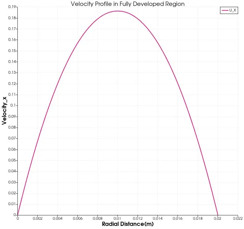 In the fully developed region the flow profile is a proper parabolic profile with highest flow velocity at the center of the pipe.
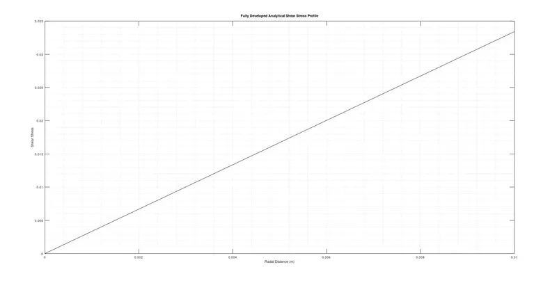
Shear Stress Profile in fully developed region :
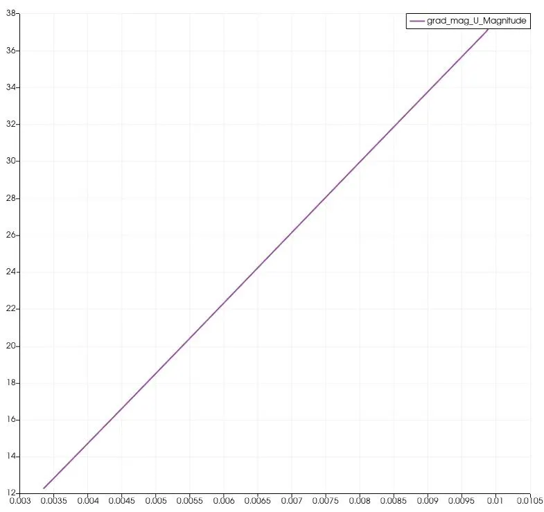
Validating the numerical result with analytical result at fully developed Region.
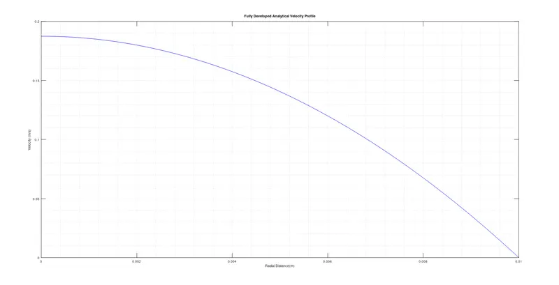
Calculating Analytical Velocity and Shear Stress Profile in Fully Developed Region.
clear all
close all
clc
d = 0.02;
r = d/2;
re = 2100;
mu = 0.891e-3;
rho = 997.13;
v_avg = 0.09373;
v_max = 2*v_avg;
R = linspace(0,r,105);
%Analytical Proof for Hydrodynamic Entrance Lenght
L_h = 0.06*re*d;
fprintf('Analytical Hydrodynamic Entrance Lenght = %f',L_h);
%Validating analytical and numerical velocity profile and shear stress profile
%at fully developed region
for i = 1:length(R)
u(i) = 2*v_avg*(1-(R(i)^2/r^2));
tau(i) = 2*mu*v_max*(abs(R(i)))/r^2;
end
plot(R,u,'b');
xlabel('Radial Distance(m)');
ylabel('Velocity (m/s)');
title('Fully Developed Analytical Velocity Profile');
grid minor;
plot(R,tau,'k');
xlabel('Radial Distance (m)');
ylabel('Shear Stress');
title('Fully Developed Analytical Shear Stress Profile');
grid minor;  Analytical Hydrodynamic Entrance lenght.
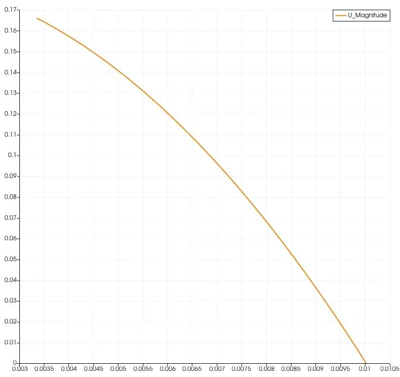
Comparing Numerical and Analytical of Velocity and Shear stress Profile.
Velocity Profile Analytical v/s Numerical :
Shear Stress Profile Analytical v/s Numerical :
Conclusions :
- Flow through pipe is very important engineering problem that is used for heating and cooling application and also for fluid distribution network.
- The flow inside the pipe occurs due to the pressure difference.
- Hagen-Poisuelles equation states that the pressure difference of the flow is directly porportional to the fluid viscoisty and inversely proportional to the sqaure of diameter.
- The calulation of pressure difference is key aspect in order to calculate the power requirement for the pump.
- For laminar flow through a pipe at the very entrance the flow is undisturbed and stable.
- After the entrance the flow at the wall comes to stop due to no-slip condition,that in turn slows down the adjecent fluid layer.This creates boundary layer in the radial direction.
- This profile after a certain distance travelling downstream become parabolic in shape.That is the flow velocity changes in the radial direction and becomes constant in the centre of the pipe.
- As the flow velocity remains constant in the hydrodynamic fully developed region the shear stress also remains constant in the region,as shear stress depend on the velocity gradient.
- The pressure drop constantly drops along the flow due to viscosity of the flow.