Week 7 - Auto ignition using Cantera

Aim: Solving the Ignition Delay of Methane fuel using Cantera in Python. Plotting the variation of ignition delay with variation of temperature and pressure values. Obtaining the molar concentration of elements 'h2o, o2 and oh' and plotting the graph of both cases.

Objective: Part1:-

simulate the Auto Ignition Time for Methane under the following conditions, (simulation time = 10 secs)

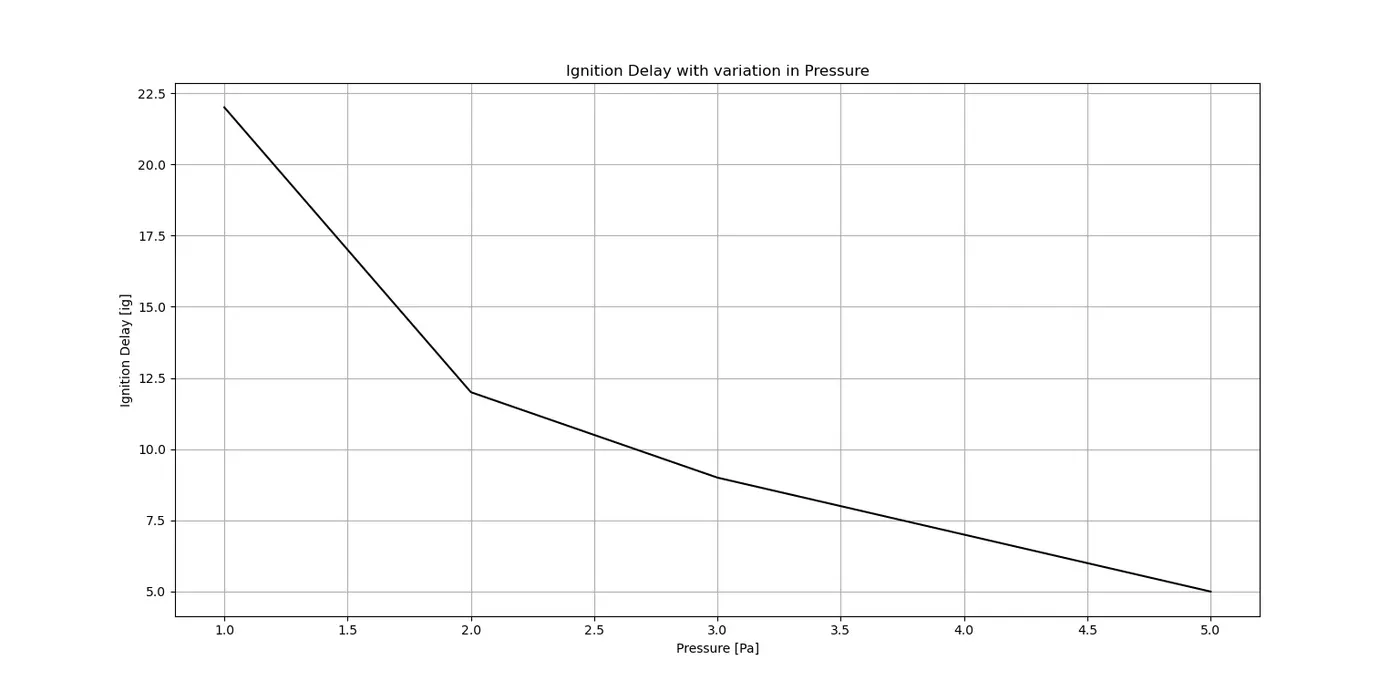
• Plot the variation of Auto Ignition time of Methane with a constant temperature of 1250K and pressure varying from 1 to 5 atm.
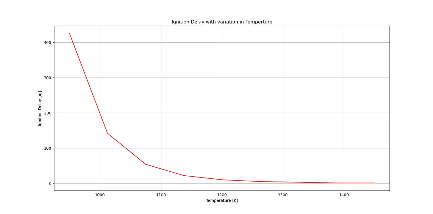
• Plot the variation of Auto Ignition time of Methane with a constant pressure of 5 atm and temperature varying from 950K to 1450K

Part2:-

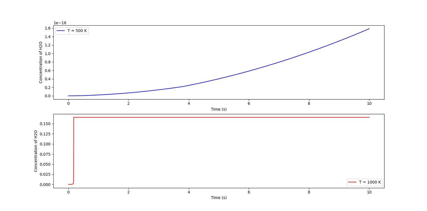
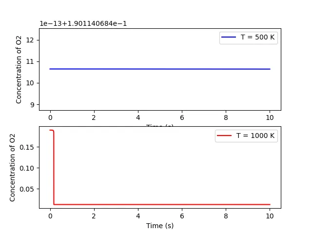
Further, observe and print the rate of change of molar concentrations of the given elements "H2O, O2, OH" with respect to the time, (simulation time = 10 secs)

Explain the behavior of the graph for 2 cases,

• When Temperature is 1000K and pressure 5 bar
• When Temperature is 500K and pressure 5 bar

Theory: Auto Ignition:-

Auto ignition is defined as the self ignition of the fuel+air composition mixture without any external ignitione source like flame or spark. This ignition happens spontaneously under right condition. The auto ignition temperature also known as knidling point, of a substance is the lowest temperature at which the fuel spontaneously ignites at room temperature. This temperature is required to provide the activation energy for combustion.

Ignition Delay(`i_g`) :-

Ignition delay (`i_g`) is defined as the time required for the ignition to take place compltely to combust the fuel. Ignition Delay depends on temperature, pressure as well as composition of fuel and air mixture. The delay in ignition is usually a very small value, considered in microseconds.

Longer ignition delay has effects on engine performance. Longer ignition delay can lead to:

1. Decreased engine efficiency.
2. Emissions of soot
3. Increased emissions of NOx
4. Increase in noise and vibration.

The ignition delay also varies with different initial temperature values also. For low temperature values the ignition delay is higher and for high temperature values the ignition delay is lower. That is for low temperature value it takes more time for fuel to ignite than higher temperature values.
While solving numerically, the ignition delay is calculated at temperture when the initial temperature becomes
(initial temperute + 400K).

There is also an abnormal behavior with the relation of ignition delay and temperature. Usually higher temperature value relates to lower ignition delay. But in certain operating conditons this relation is not obeyed and the ignition delay starts rising with increase in temperture this phenomena is known as Negative Temperature Coefficient (NTC).

Reactor class of Cantera:-

As we have to carry out the combustion of the Fuel Methane with oxidizer Air in a closed system, we have to created this closed system first. But the Cantera library contains a class called Reactor. This reactor can be specified with inlets and outlets, mass flow rates or without inlet and outlet. This class is used to compute Combustion, Reactor design and optimization, Pyrolysis, Catalysis.

Also there are different types of reactor types we can use to simulate the real world like problem:

1. Reactor : A homogeneous zero-dimensional reactor. By default, they are closed (no inlets or outlets), have fixed volume, and have adiabatic, chemically-inert walls. These properties may all be changed by adding appropriate components such as Wall, MassFlowController and Valve.
2. IdealGasReactor : it is a constant volume, zero dimensional reactor for ideal gas mixtures.
3. ConstPressureReactor : constant pressure, zero dimensional reactor. The volume of reactor changes as function of time to keep pressure constant.
4. IdealGasConstPreussreReactor : A homogeneous, constant pressure, zero-dimensional reactor for ideal gas mixtures. The volume of the reactor changes as a function of time in order to keep the pressure constant.

For our case of simulation we will use the Reactor class, as it matches with our simulation condition the best.

Now we have created the Reactor and set all necessary operating conditons, we need to solve the chemical reation inside the Reactor. To complete this purpose we will use the ReactionNet class of Cantera.
This class is used to compute any chemical reaction for a single reactor or multiple chain of reactors. With aid of this class we can add different mixtures reactors and solve them together.

When we solve transient problem like this in Cantera, remember that the time value we define is the total end time value rather than the time-steps size. The time-steps size is calcualted by Cantera itself. This total end time value we define is the definite value/ upper limit for the integration in time to solve the thermo state of the reactor.

Code:

Code for Ignition Delay for variaton temperature and variation pressure:

"""
Creating a function which will take T,P and specied dictonary as input
based on that constant temperature and constant pressure Ignition delay will be calculated.

The methane+air mixture of stoichiometric composition is used.

Reactor and ReactorNet class are introduced in completing this simualtion
"""
import cantera as ct
import numpy as np
import matplotlib.pyplot as plt

###function iG takes T, P and species directory as input of function

def iG(T, P, species_dic):

    # gas     = ct.Solution('gri30.yaml')
    # gas.TPX = T, P, species_dic
    Ig        = []                         #emptry array that will be output time value for ignition delay


    gas     = ct.Solution('gri30.yaml')
    gas.TPX = T, P, species_dic

    r       = ct.IdealGasReactor(gas)

    sim1     = ct.ReactorNet([r])
    time     = 0.0
    states   = ct.SolutionArray(gas, extra=['time_in_ms', 't'])

    for i in range(1000):
        time += 1e-3
        sim1.advance(time)
        states.append(r.thermo.state, time_in_ms = time*1e3, t = time)

    for j in range (len(states.T)):
        if states[j].T >= (1250+400):
            Ig.append(states.time_in_ms[j])

            break
    return Ig


###Inputs for the Option 1 iG
T = 1250
P_arr = np.linspace(1,5,5)
species = {'CH4':1, 'O2':2, 'N2': 7.52}

cnst_P = np.zeros(len(P_arr))

for i in range(len(P_arr)):
    P = P_arr[i]*101325

    cnst_P[i] = iG(T, P, species)[0]

plt.plot(P_arr, cnst_P, 'k')
plt.xlabel('Pressure [Pa]')
plt.ylabel('Ignition Delay [ig]')
plt.title('Ignition Delay with variation in Pressure')
plt.grid('major')
plt.show()

T_arr = np.linspace(950,1450,9)
P = 5*101325

cnst_T = np.zeros(len(T_arr))

for i in range(len(T_arr)):
    T = T_arr[i]

    cnst_T[i] = iG(T, P, species)[0]

plt.plot(T_arr, cnst_T, 'r')
plt.xlabel('Temperature [K]')
plt.ylabel('Ignition Delay [ig]')
plt.title('Ignition Delay with variation in Temperture')
plt.grid('major')
plt.show()

Result for Ignition Delay vs varied pressure:

Result for Ignition Delay vs varied temperature:

Conclusion for Part 1:

• For the case of constant temperature and varied pressure from 0 to 5 atm.
  
  • The Ignition Delay for variation in pressure value is computed.
  • As the pressure increases the auto ignition delay time decreases.
  • The reason for decrease in ignition delay with increase in pressure is due to, Increase in Pressure increases in the concentration of the radicals that are responsible for initiating the combustion reaction. Radicals are highly reactive chemical species that have at least one unpaired electron. They are formed during the initial stages of the combustion reaction and play a key role in propagating the flame.
• For the case of constant pressure and varied temperature from 950 to 1450 K.
  As the initial temperature increases the value of ignition delay decreases.
  As temperture increases it increases the rate of chemical reactions. At high rate of chemical reactions the reactants reacts more quickly and combust.
  Higher temperature increases the average kinetic energy of the reactant molecules, which makes it more likely that they will have enough energy to overcome the activation energy barrier and react.

Part 2:

Printing rate of change of molar concentration of elements 'oh, h20 and o2'.

Code:

import sys
import numpy as np 
import cantera as ct
import matplotlib.pyplot as plt
gas = ct.Solution('gri30.yaml')

T = [500,1000]
P = 5*101325



#create gas object
for i in range(len(T)):
	
	gas.TPX = T[i],P,{'CH4':1,'O2':2,'N2':7.52}

	#create reactor object that takes in the gas object
	r = ct.IdealGasReactor(gas)
	sim = ct.ReactorNet([r])

	time = 0.0
	states500 = ct.SolutionArray(gas, extra = ['time_in_ms','t'])
	states1000 = ct.SolutionArray(gas, extra = ['time_in_ms','t'])


	if i == 0:
		for n in range(10000):
			time+= 1e-3
			sim.advance(time)
			states500.append(r.thermo.state,time_in_ms = time*1e3, t = time)
	plt.figure(1)
	plt.subplot(2,1,1)
	plt.plot(states500.t,states500.X[:,gas.species_index('H2O')],color = 'blue')
	plt.xlabel('Time (s)')
	plt.ylabel('Concentration of H2O')
	plt.legend(['T = 500 K'])

	plt.figure(2)
	plt.subplot(2,1,1)
	plt.plot(states500.t,states500.X[:,gas.species_index('O2')],color = 'blue')
	plt.xlabel('Time (s)')
	plt.ylabel('Concentration of O2')
	plt.legend(['T = 500 K'])

	plt.figure(3)
	plt.subplot(2,1,1)
	plt.plot(states500.t,states500.X[:,gas.species_index('OH')],color = 'blue')
	plt.xlabel('Time (s)')
	plt.ylabel('Concentration of OH')
	plt.legend(['T = 500 K'])

	if i == 1:
		for n in range(10000):
			time+= 1e-3
			sim.advance(time)
			states1000.append(r.thermo.state,time_in_ms = time*1e3, t = time)
		
	plt.figure(1)
	plt.subplot(2,1,2)
	plt.plot(states1000.t,states1000.X[:,gas.species_index('H2O')],color = 'red')
	plt.xlabel('Time (s)')
	plt.ylabel('Concentration of H2O')
	plt.legend(['T = 1000 K'])

	plt.figure(2)
	plt.subplot(2,1,2)
	plt.plot(states1000.t,states1000.X[:,gas.species_index('O2')],color = 'red')
	plt.xlabel('Time (s)')
	plt.ylabel('Concentration of O2')
	plt.legend(['T = 1000 K'])

	plt.figure(3)
	plt.subplot(2,1,2)
	plt.plot(states1000.t,states1000.X[:,gas.species_index('OH')],color = 'red')
	plt.xlabel('Time (s)')
	plt.ylabel('Concentration of OH')
	plt.legend(['T = 1000 K'])



plt.show()

H2O concentration of mole:

O2 concentration of mole :

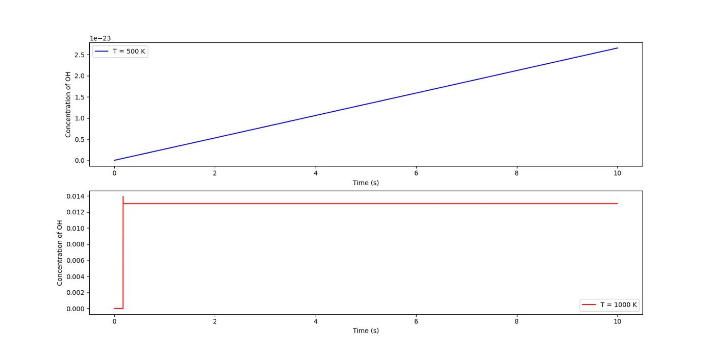
OH concentration of mole:

Conclusion for part 2:

The concentration of O2 is seem to be constant at 500K throughtout the 10s simualtion time, indicating that combustion dosent took place at 500K. For the same temperature the concentration of H2O and Oh seems to be increasing at very different pace. This changes may be depend upon the chemical kinetics of the reaction at that temperature.

At 1000K, Oh and H2O, a sudden increase in the concentration is observed that ignition took place that results in decrease in reactants and very sudden and sharp increase in the byproducts of the reaction. The decrease in the O2 is seen which proofs that ignition took place and reactants starts to convert to products.