Week 3 - Adiabatic Flame Temperature calculation
Aim:- Compute the Adiabatic Flame Temperature for constant-pressure, constant volume processes. Plot the graph for the AFT with variation in Equivalence Ratio, Hydrocarbon Fuel with constant Carbon atoms and with variation in Carbon atoms.
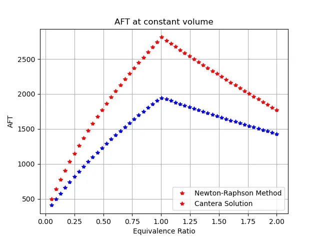
Objective:- 1. AFT variation with Equivalence Ratio in constant-volume process from Python and Cantera.
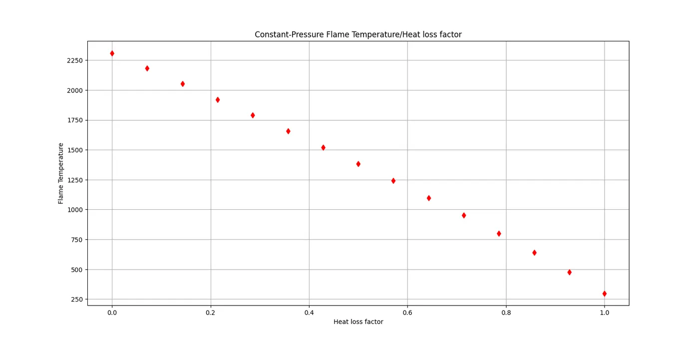
2. Flame Temperature variation with Heat loss in constant-pressure process.
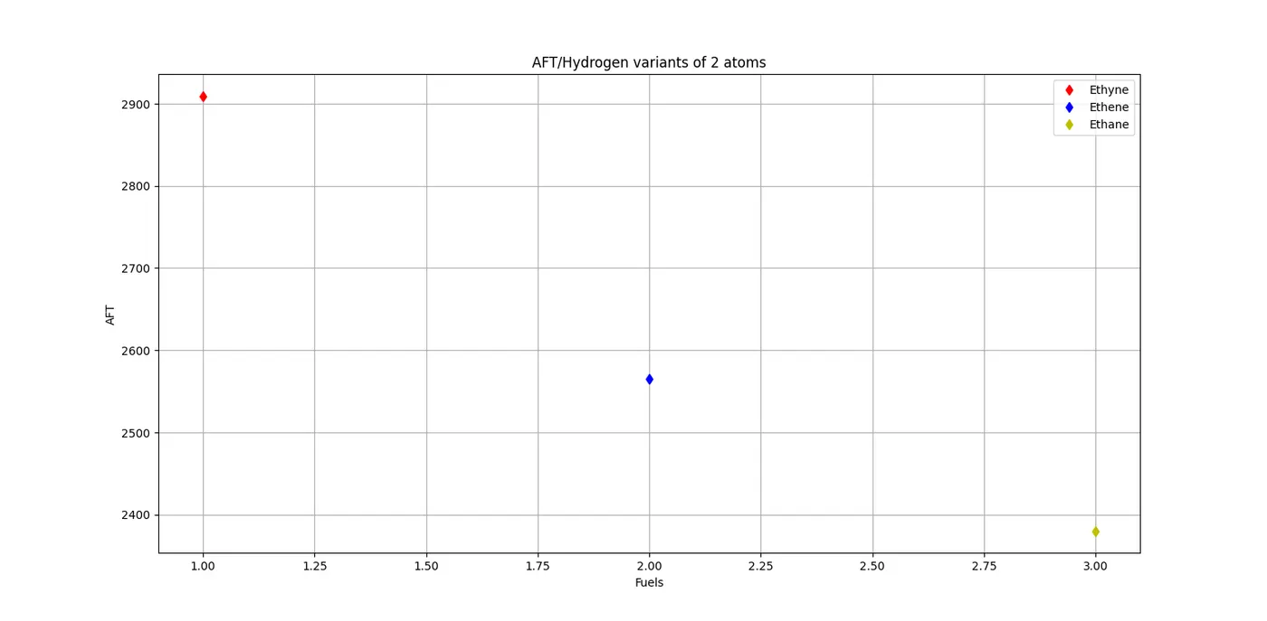
3. AFT variation with respect to Alkane, Alkene and Alkyne.
4. AFT variation with respect to number of Carbon atom chains.
Theory:-
- Adiabatic Flame Temperature : In study of combustion, Adiabatic Flame Temperature is the temperature reached by the products of combustion in an ideal state which considers no Heal Loss to the surrounding. This Temperature is the upper bound temperature of any fuel that is reached in actual processes.
There are two types of Adiabatic Flame Temperature: constant-volume and constant-pressure. The AFT is higher for the constant-volume process,due to no work is done by the flame on the surrounding in constant-volume process. Where in constant-pressure process the work is done on the surrounding. - Stoichiometry : The Stoichiometry ratio or Stoichiometry amount is that ratio which provides the compelte utilization of reactants(oxygen and Fuel) to burn and produce products with no unburned reactants. For a complete Stoichiometric combustion equation the Equivalence Ratio is 1.
- Equivalence Ratio : It is defined as the ratio of actual (Fuel/Air) to the Stoichiometric (Fuel/Air) ratio. The Equivalence ration affects the efficiency of combustion and generation of harmful products with unburned gases also. The Equivalence Ratio is represents as Φ and it depends on the actual (Fuel/Air) ratio.
If Φ < 1>
If Φ = 1, Stoichiometric Mixture, the quantity of Fuel is in exact amount with quantity of Oxidizer. No byproducts, compelte combustion.
If Φ>1, Lean Mixture, the quantity of air is greater than the quantity of fuel. Lean Mixtures are efficient but may cause higher temperatures and creates Nitriogen Oxides. - Newton Raphson's Method : The Newton-Raphsons method is a root-finding algorithm that producess better approximation of the roots of the real-valued function. The calcualtion starts with taking the function, its first derivative, an initial guess value of the root and the formula for calculating the value of root is,
`x_1 = x_0 - f(x_0)/(f'(x_0))`
The equation is the better approximation than the x_0.
The idea is to start the value with an initial guess and then approximate the function at guess value by its tangent line. This x-intercept is typically a better value than the original guess value.
Procedure:-
1. Adiabatic Flame Temperature variation with Equivalence Ratio (constant-volume process):
- Python code and Results:
"""
    Python code for solving AFT of constant-volume process.
    Plotting Equivalave ratio v/s AFT for python code and from cantera.

    Lean Mixture :
        CH4 + 2/phi*(O2 + 3.76N2) -> aCO2 + bH2O + 7.62/phiN2 + (2/phi-2)O2
        with a = 1, b = 2.
    Rich Mixture :
        CH4 + 2/phi*(O2 + 3.76N2) -> (4/phi-3)CO2 + bH2O + 7.62/phiN2 + (4-(4/phi))CO

    The AFT is solved using Newton-Raphson method in Python
"""

import cantera as can
import matplotlib.pyplot as plt
import numpy as np

Tstp = 298.15 #K
R    = 8.314  #J/molK

#defining the enthalpy function
def H(T, coeffs):
    a1 = coeffs[0]
    a2 = coeffs[1]
    a3 = coeffs[2]
    a4 = coeffs[3]
    a5 = coeffs[4]
    a6 = coeffs[5]

    #NASA polynomials for calculating the enthalpy
    return (a1 + a2*T/2 + a3*pow(T,2)/3 + a4*pow(T,3)/4 + a5*pow(T,4)/5 + a6/T)*R*T

#The coefficients values for lower temperatures for each species
ch4_coeff_l = [5.14987613E+00, -1.36709788E-02, 4.91800599E-05, -4.84743026E-08, 1.66693956E-11, -1.02466476E+04, -4.64130376E+00]
o2_coeff_l = [3.78245636E+00, -2.99673416E-03, 9.84730201E-06, -9.68129509E-09, 3.24372837E-12, -1.06394356E+03, 3.65767573E+00]
n2_coeff_l = [0.03298677E+02, 0.14082404E-02, -0.03963222E-04, 0.05641515E-07, -0.02444854E-10, -0.10208999E+04, 0.03950372E+02]
# Coefficients for the NASA polynomial for high temperatures
co2_coeff_h = [3.85746029E+00, 4.41437026E-03, -2.21481404E-06, 5.23490188E-10, -4.72084164E-14, -4.87591660E+04, 2.27163806E+00]
h2o_coeff_h = [3.03399249E+00, 2.17691804E-03, -1.64072518E-07, -9.70419870E-11, 1.68200992E-14, -3.00042971E+04, 4.96677010E+00]
n2_coeff_h = [0.02926640E+02, 0.14879768E-02, -0.05684760E-05, 0.10097038E-09, -0.06753351E-13, -0.09227977E+04, 0.05980528E+02]
co_coeff_h = [2.71518561E+00, 2.06252743E-03, -9.98825771E-07, 2.30053008E-10, -2.03647716E-14, -1.41518724E+04, 7.81868772E+00]
o2_coeff_h =  [3.28253784E+00, 1.48308754E-03, -7.57966669E-07, 2.09470555E-10, -2.16717794E-14, -1.08845772E+03, 5.45323129E+00]

#Defining the function for calculating the enthalpies with temperature value as input using the constant volume process
#for different values of phi
def f(T,phi):
    #calculating the reactants enthalpy
    h_ch4_r = H(Tstp,ch4_coeff_l)
    h_o2_r  = H(Tstp,o2_coeff_l)
    h_n2_r  = H(Tstp,n2_coeff_l)

    #calculating products enthalpy
    h_co2_p = H(T,co2_coeff_h)
    h_h2o_p = H(T,h2o_coeff_h)
    h_n2_p  = H(T,n2_coeff_h)
    h_co_p  = H(T,co_coeff_h)
    h_o2_p  = H(T,o2_coeff_h)

    #calculating the coefficients different Equaivalence Ratio
    if phi <= 1:    #Lean Mixture
        a = 1
        b = 2
        c = 7.62/phi
        d = (2/phi) - 2

        #calculating the enthalpy of products respective to Equivalence Ratio
        H_products = a*h_co2_p + b*h_h2o_p + c*h_n2_p + d*h_o2_p

        #calculating the number of moles
        N_p = a + b + c + d

    elif phi == 1:    #Stoichiometric Mixture
        a = 1
        b = 2
        c = 7.52

        #calculating the enthalpy of products respective to Equivalence Ratio
        H_products = a*h_co2_p + b*h_h2o_p + c*h_n2_p

        #calculating the number of moles
        N_p = a + b + c

    else:    #Rich Mixture
        a = (4/phi) - 3
        b = 2
        c = 7.52/phi
        d = 4 - (4/phi)

        #calculating the enthalpy of products respective to Equivalence Ratio
        H_products = a*h_co2_p + b*h_h2o_p + c*h_n2_p + d*h_co_p

        #calculating the number of moles
        N_p = a + b + c + d

    #Enthalpy of Reactants
    H_reactants = h_ch4_r + (2/phi)*(h_o2_r + (3.76*h_n2_r))

    #number of moles of reactants
    N_r = 1 + (2/phi) + 3.76*(2/phi)

    #calculating the function
    return (H_products - H_reactants - R*(N_p*T -(N_r*Tstp)))

def fprime(T):
    return (f(T+1e-5,phi[i]) - f(T,phi[i]))/1e-5


#values of phi for a range from 0.5 to 2
phi = np.linspace(0.05,2.0,50)
#Defining the values for N-R method
t_guess = 1500
alpha = 0.2
tol = 1e-3
ct = 0

for i in range(len(phi)):
    while(abs(f(t_guess,phi[i])) > tol):
        t_guess = t_guess - alpha*(f(t_guess,phi[i])/fprime(t_guess))
        ct = ct+1

    plt.plot(phi[i],t_guess,'r*')


#print(t_guess)
#print(ct)

#Cantera Solution
T_ct = []

for j in range(len(phi)):
    gas = can.Solution('gri30.yaml')
    gas.TPX = Tstp,101325,{'CH4':1, 'O2':2, 'N2':7.52}
    gas.set_equivalence_ratio(phi[j],'CH4', 'O2:1, N2:7.52')
    gas.equilibrate('UV', 'auto')
    T_ct.append(gas.T)
    plt.plot(phi[j],gas.T,'-b*')

plt.xlabel('Equivalence Ratio')
plt.ylabel('AFT')
plt.title('AFT at constant volume')
plt.legend(['Newton-Raphson Method', 'Cantera Solution'], loc = 'lower right')
plt.grid(which = 'both')
plt.show()
2. Flame Temperature variation with Heat Loss (constant-pressure process):
Consider a constant pressure reactor with heat loss. The reactor is set initially at STP conditions. The heat loss of the combustion is given by this formula:
The heat loss of the reaction can be controlled by multiplying the maximum heat loss equation to the heat_loss_factor.
The chemical reaction of the combustion is: `CH_4 + 2(O_2+3.76N_2) ->CO_2 + 2H_2O+7.62N_2`
The reaction is stoichiometry no byproducts will be created. The formula for root finidng the Temperature is given as
(H_products - H_reactants) - h_loss*(H_products_STP - H_reactants)
The python logic is used to calculate the Temperature of the heat loss. The Newton-Raphson methods is used to calcualte the value of temperature as the above equation is equals to 0.
- Python Code for calcualting Flame Temperature and plot.
"""
    Solving constant pressure AFT with heat loss.
    The initial conditions are at STP

    Vary heat loss by multiplying with heat loss factor and plot temperature agianst it.

    Combustion reaction
        CH4 + 2(O2 + 3.76N2) -> CO2 + 2H2O + 7.62N2
    Stoichiometric equation

    The maximum heat loss by the combustion is varied by the 'h_loss' factor
"""

import matplotlib.pyplot as plt
import numpy as np

Tstp = 298.15 #K
R    = 8.314  #J/molK

#defining the enthalpy function
def H(T, coeffs):
    a1 = coeffs[0]
    a2 = coeffs[1]
    a3 = coeffs[2]
    a4 = coeffs[3]
    a5 = coeffs[4]
    a6 = coeffs[5]

    #NASA polynomials for calculating the enthalpy
    return (a1 + a2*T/2 + a3*pow(T,2)/3 + a4*pow(T,3)/4 + a5*pow(T,4)/5 + a6/T)*R*T

#The coefficients values for lower temperatures for each species
ch4_coeff_l = [5.14987613E+00, -1.36709788E-02, 4.91800599E-05, -4.84743026E-08, 1.66693956E-11, -1.02466476E+04, -4.64130376E+00]
o2_coeff_l = [3.78245636E+00, -2.99673416E-03, 9.84730201E-06, -9.68129509E-09, 3.24372837E-12, -1.06394356E+03, 3.65767573E+00]
n2_coeff_l = [0.03298677E+02, 0.14082404E-02, -0.03963222E-04, 0.05641515E-07, -0.02444854E-10, -0.10208999E+04, 0.03950372E+02]
# Coefficients for the NASA polynomial for high temperatures
co2_coeff_h = [3.85746029E+00, 4.41437026E-03, -2.21481404E-06, 5.23490188E-10, -4.72084164E-14, -4.87591660E+04, 2.27163806E+00]
h2o_coeff_h = [3.03399249E+00, 2.17691804E-03, -1.64072518E-07, -9.70419870E-11, 1.68200992E-14, -3.00042971E+04, 4.96677010E+00]
n2_coeff_h = [0.02926640E+02, 0.14879768E-02, -0.05684760E-05, 0.10097038E-09, -0.06753351E-13, -0.09227977E+04, 0.05980528E+02]
co_coeff_h = [2.71518561E+00, 2.06252743E-03, -9.98825771E-07, 2.30053008E-10, -2.03647716E-14, -1.41518724E+04, 7.81868772E+00]
o2_coeff_h =  [3.28253784E+00, 1.48308754E-03, -7.57966669E-07, 2.09470555E-10, -2.16717794E-14, -1.08845772E+03, 5.45323129E+00]


#Defining the function for calculating the enthalpies for value of T
#with different value of h_loss
def f(T,h_loss):
    #Enthalpy of Reactants
    h_ch4_r = H(Tstp,ch4_coeff_l)
    h_o2_r  = H(Tstp,o2_coeff_l)
    h_n2_r  = H(Tstp,n2_coeff_l)

    #Enthalpy of Products
    h_co2_hp = H(T,co2_coeff_h)
    h_h2o_hp = H(T,h2o_coeff_h)
    h_n2_hp  = H(T,n2_coeff_h)

    #Enthalpy of Products at STP
    h_co2_sp = H(Tstp,co2_coeff_h)
    h_h2o_sp = H(Tstp,h2o_coeff_h)
    h_n2_sp  = H(Tstp,n2_coeff_h)

    H_reactants = h_ch4_r + 2*h_o2_r + 7.62*h_n2_r

    H_products_T = h_co2_hp + 2*h_h2o_hp + 7.62*h_n2_hp

    H_products_Tstp = h_co2_sp + 2*h_h2o_sp + 7.62*h_n2_sp

    return (H_products_T - H_reactants) - h_loss*(H_products_Tstp - H_reactants)

def fprime(T):
    return (f(T+1e-6, h_loss[i]) - f(T, h_loss[i]))/1e-6

h_loss = np.linspace(0.0,1.0,15)

T_g   = 1500
alpha = 0.2
tol   = 1e-4
ct    = 0

for i in range(len(h_loss)):

    while (abs(f(T_g,h_loss[i])) > tol):
        T_g = T_g - alpha*(f(T_g,h_loss[i])/fprime(T_g))
        ct  = ct + 1

    plt.plot(h_loss[i],T_g,'rd')

print(T_g)
print(ct)

plt.xlabel('Heat loss factor')
plt.ylabel('Flame Temperature')
plt.title('Constant-Pressure Flame Temperature/Heat loss factor')
plt.grid(which='both')
plt.show()- Functions are created for calculating the Enthalpy and the equation in question.
- The enthalpy function, defined as H takes in the value of Temperature and coefficients values that are passed as list. In the function the coefficients are defined as a1,a2,a3,a4,a5,a6 that are equal to the coeff of the paramters. This function than returns the Enthalpy that is than calculated by using the NASA Polynomial equation for enthalpy.
- The next function takes in the value of Temperature and the heat loss factor as input. The enthalpies of the reactants and products are calculated species wise and than all together are summed by multiplying with thier molar quantity.
- The fprime function is the first derivative of the Temperature, as shown in the Newton-Raphson method. This value is calcualted using the Forward Differencing Scheme.
- Using the linspace() command of the Numpy Library of Python, equally spaced h_loss values are generated from 0 to 1
- The necessary variables like initial guess value for temperature, the relaxation factor(alpha),(ct) counter and the tolerance values are defined.
- Then the Temperature value is calculated for the range of the h_loss factor. For each h_loss factor value, the guess value of Temperature is evaluated with the tolerance and while the value will be greater than the tolerance the Newton-Raphson formula will executed for calculating the better approximation and the counter ct will be updated by 1.
- Then in the for loop, the graph for h_loss/Temperature is plotted for each h_loss value.

Plot:
3. Adiabatic Flame Temperature with respect to Alkane, Alkene and Alkyne:
The in question Alkyne, Alkene and Alkane are Ethyne(C2H2), Ethene(C2H4) and Ehtane(C2H6) respectively. The combustion equations are Stoichiometric. The reaction is given as follows:
Ethyne: `C_2H_2 + 2.5(O_2+3.76N_2)->2CO_2+H_2O+9.4N_2`
Ethene: `C_2H_4+3(O_2+3.76N_2)->2CO_2+2H_2O+11.28N_2`
Ethane: `C_2H_6+3.5(O_2+3.76N_2)->2CO_2 + 3H_2O+13.16N_2`
The general Stoichiometric coefficient for all three hydrocarbons is x+y/4
- Python code for calculation and graph plotting:
"""
    Calculating the AFT for constant pressure.
    Calculating the AFT for different Hydrocarbon Fuels with variant in Hydrogen atoms.

    Hydrocarbon fuels : [C2H2, C2H4, C2H6]

    The list of fuel in past as input for f(T) function and
    enthalpies are calculated for each fuel for stoichiometric combustion reactions.

        Ethyne: C2H2 + 2.5(O2 + 3.76N2) -> 2CO2 + H2O + 9.4N2
        Ethene: C2H4 + 3(O2 + 3.76N2) -> 2CO2 + 2H2O + 11.28N2
        Ethane: C2H4 + 3.5(O2 + 3.76N2) -> 3CO2 + 2H2O + 13.16N2
"""

#import cantera as ct
import matplotlib.pyplot as plt
import numpy as np

Tstp = 298.15 #K
R    = 8.314  #J/molK

#defining the enthalpy function
def H(T, coeffs):
    a1 = coeffs[0]
    a2 = coeffs[1]
    a3 = coeffs[2]
    a4 = coeffs[3]
    a5 = coeffs[4]
    a6 = coeffs[5]

    #NASA polynomials for calculating the enthalpy
    return (a1 + a2*T/2 + a3*pow(T,2)/3 + a4*pow(T,3)/4 + a5*pow(T,4)/5 + a6/T)*R*T

#The coefficients values for lower temperatures for each species
c2h6_coeff_l = [4.29142492E+00,-5.50154270E-03 ,5.99438288E-05,-7.08466285E-08 ,2.68685771E-11,-1.15222055E+04 ,2.66682316E+00]
c2h4_coeff_l = [3.95920148E+00,-7.57052247E-03 ,5.70990292E-05,-6.91588753E-08 ,2.69884373E-11 ,5.08977593E+03 ,4.09733096E+00]
c2h2_coeff_l = [8.08681094E-01, 2.33615629E-02,-3.55171815E-05, 2.80152437E-08,-8.50072974E-12, 2.64289807E+04, 1.39397051E+01]
o2_coeff_l = [3.78245636E+00, -2.99673416E-03, 9.84730201E-06, -9.68129509E-09, 3.24372837E-12, -1.06394356E+03, 3.65767573E+00]
n2_coeff_l = [0.03298677E+02, 0.14082404E-02, -0.03963222E-04, 0.05641515E-07, -0.02444854E-10, -0.10208999E+04, 0.03950372E+02]
# Coefficients for the NASA polynomial for high temperatures
co2_coeff_h = [3.85746029E+00, 4.41437026E-03, -2.21481404E-06, 5.23490188E-10, -4.72084164E-14, -4.87591660E+04, 2.27163806E+00]
h2o_coeff_h = [3.03399249E+00, 2.17691804E-03, -1.64072518E-07, -9.70419870E-11, 1.68200992E-14, -3.00042971E+04, 4.96677010E+00]
n2_coeff_h = [0.02926640E+02, 0.14879768E-02, -0.05684760E-05, 0.10097038E-09, -0.06753351E-13, -0.09227977E+04, 0.05980528E+02]
co_coeff_h = [2.71518561E+00, 2.06252743E-03, -9.98825771E-07, 2.30053008E-10, -2.03647716E-14, -1.41518724E+04, 7.81868772E+00]
o2_coeff_h =  [3.28253784E+00, 1.48308754E-03, -7.57966669E-07, 2.09470555E-10, -2.16717794E-14, -1.08845772E+03, 5.45323129E+00]


#Defining the function for calculating the enthalpies with temperature value as input using the constant pressure process
#for different values of fuels
def f(T,fuels):
    #calculating the reactants enthalpy
    h_c2h2_r = H(Tstp,c2h2_coeff_l)
    h_c2h4_r = H(Tstp,c2h4_coeff_l)
    h_c2h6_r = H(Tstp,c2h6_coeff_l)
    h_o2_r   = H(Tstp,o2_coeff_l)
    h_n2_r   = H(Tstp,n2_coeff_l)

    #calculating the products enthalpy
    h_co2_p = H(T,co2_coeff_h)
    h_h2o_p = H(T,h2o_coeff_h)
    h_n2_p  = H(T,n2_coeff_h)

    if fuels == 1:  #Ethyne
        H_reactants = h_c2h2_r + 2.5*h_o2_r + 9.4*h_n2_r
        H_products  = 2*h_co2_p + h_h2o_p + 9.4*h_n2_p

    elif fuels == 2:    #Ethene
        H_reactants = h_c2h4_r + 3*h_o2_r + 11.28*h_n2_r
        H_products  = 2*h_co2_p + 2*h_h2o_p + 11.28*h_n2_p

    else:               #Ethane
        H_reactants = h_c2h6_r + 3.5*h_o2_r + 13.16*h_n2_r
        H_products  = 2*h_co2_p + 3*h_h2o_p + 13.16*h_n2_p

    return H_products - H_reactants

def fprime(T):
    return (f(T+1e-6,fuels[i])/f(T,fuels[i]))/1e-6


fuels = np.linspace(1,3,3)

t_g   = 1500
alpha = 0.5
tol   = 1e-4
ct    = 0
AFT = []

for i in range(len(fuels)):
    while (abs(f(t_g,fuels[i])) > tol):
        t_g = t_g - alpha*(f(t_g,fuels[i])/fprime(t_g))
        ct = ct+1

    AFT.append(t_g)

    if fuels[i] == 1:
        plt.plot(fuels[i], t_g, 'rd')
        print('Ethyne AFT:',AFT[0])

    if fuels[i] == 2:
        plt.plot(fuels[i], t_g, 'bd')
        print('Ethene AFT:', AFT[1])

    if fuels[i] == 3:
        plt.plot(fuels[i], t_g, 'yd')
        print('Ethane AFT', AFT[2])


plt.xlabel('Fuels')
plt.ylabel('AFT')
plt.title('AFT/Hydrogen variants of 2 atoms', loc='center')
plt.legend(['Ethyne', 'Ethene', 'Ethane'], loc = 'upper right')
plt.grid(which='both')
plt.show()
#print(t_g)
#print(ct)- The first step of defining the Enthlapy function is same as above codes.
- The fuels variable passed as input for the 'f' function is the linspace from 1 to 3. Where 1 = Ethyne, 2 = Ethene and 3 = Ethane. This function will take this value and according the value of fuels, it will calcualte the appropriate fuel reactants and products enthalpy and will return the value of H_products - H_reactants.
- Then fprime function is defined. Then for each fuel value the tolerance value of the guessed value is checked and the formula of N-R is calulated and the plot and temperature and counter values are printed and are shown below.
- Plots and temperature values:

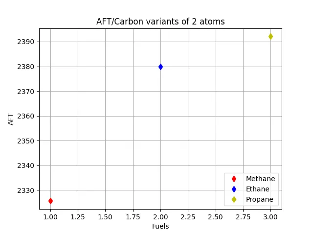
4. AFT variation with respect to Carbon atoms:
The in question variants of Carbon atome are Methane(CH4), Ethane(C2H6) and Propane(C3H8) respectively. The combustion equations are Stoichiometric. The reaction is given as follows:
Methane: `CH_4 + 2(O_2+3.76N_2)->CO_2+2H_2O+7.52N_2`
Ethane: `C_2H_6+3.5(O_2+3.76N_2)->2CO_2+3H_2O+13.6N_2`
Propane: `C_3H_8+5(O_2+3.76N_2)->3CO_2 + 4H_2O+18.8N_2`
The general Stoichiometric coefficient for all three hydrocarbons is x+y/4
- Python code and results:
"""
    Calculating the AFT for constant pressure.
    Calculating the AFT for different Hydrocarbon Fuels with variant in Carbon atoms.

    Hydrocarbon fuels : [CH4, C2H6, C3H8]

    The list of fuel in past as input for f(T) function and
    enthalpies are calculated for each fuel for stoichiometric combustion reactions.

        Methane: CH4 + 2(O2 + 3.76N2) -> CO2 + 2H2O + 7.52N2
        Ethane: C2H6 + 3.5(O2 + 3.76N2) -> 2CO2 + 3H2O + 13.16N2
        Propane: C3H8 + 5(O2 + 3.76N2) -> 3CO2 + 4H2O + 18.8N2
"""

#import cantera as ct
import matplotlib.pyplot as plt
import numpy as np

Tstp = 298.15 #K
R    = 8.314  #J/molK

#defining the enthalpy function
def H(T, coeffs):
    a1 = coeffs[0]
    a2 = coeffs[1]
    a3 = coeffs[2]
    a4 = coeffs[3]
    a5 = coeffs[4]
    a6 = coeffs[5]

    #NASA polynomials for calculating the enthalpy
    return (a1 + a2*T/2 + a3*pow(T,2)/3 + a4*pow(T,3)/4 + a5*pow(T,4)/5 + a6/T)*R*T

#The coefficients values for lower temperatures for each species
ch4_coeff_l = [5.14987613E+00,-1.36709788E-02, 4.91800599E-05,-4.84743026E-08, 1.66693956E-11,-1.02466476E+04,-4.64130376E+00]
c2h6_coeff_l = [4.29142492E+00,-5.50154270E-03, 5.99438288E-05,-7.08466285E-08, 2.68685771E-11,-1.15222055E+04, 2.66682316E+00]
c3h8_coeff_l = [0.93355381E+00, 0.26424579E-01, 0.61059727E-05,-0.21977499E-07, 0.95149253E-11,-0.13958520E+05, 0.19201691E+02]
o2_coeff_l = [3.78245636E+00, -2.99673416E-03, 9.84730201E-06, -9.68129509E-09, 3.24372837E-12, -1.06394356E+03, 3.65767573E+00]
n2_coeff_l = [0.03298677E+02, 0.14082404E-02, -0.03963222E-04, 0.05641515E-07, -0.02444854E-10, -0.10208999E+04, 0.03950372E+02]
# Coefficients for the NASA polynomial for high temperatures
co2_coeff_h = [3.85746029E+00, 4.41437026E-03, -2.21481404E-06, 5.23490188E-10, -4.72084164E-14, -4.87591660E+04, 2.27163806E+00]
h2o_coeff_h = [3.03399249E+00, 2.17691804E-03, -1.64072518E-07, -9.70419870E-11, 1.68200992E-14, -3.00042971E+04, 4.96677010E+00]
n2_coeff_h = [0.02926640E+02, 0.14879768E-02, -0.05684760E-05, 0.10097038E-09, -0.06753351E-13, -0.09227977E+04, 0.05980528E+02]
co_coeff_h = [2.71518561E+00, 2.06252743E-03, -9.98825771E-07, 2.30053008E-10, -2.03647716E-14, -1.41518724E+04, 7.81868772E+00]
o2_coeff_h =  [3.28253784E+00, 1.48308754E-03, -7.57966669E-07, 2.09470555E-10, -2.16717794E-14, -1.08845772E+03, 5.45323129E+00]


#Defining the function for calculating the enthalpies with temperature value as input using the constant pressure process
#for different values of fuels
def f(T,fuels):
    #calculating the reactants enthalpy
    h_ch4_r = H(Tstp,ch4_coeff_l)
    h_c2h6_r = H(Tstp,c2h6_coeff_l)
    h_c3h8_r = H(Tstp,c3h8_coeff_l)
    h_o2_r   = H(Tstp,o2_coeff_l)
    h_n2_r   = H(Tstp,n2_coeff_l)

    #calculating the products enthalpy
    h_co2_p = H(T,co2_coeff_h)
    h_h2o_p = H(T,h2o_coeff_h)
    h_n2_p  = H(T,n2_coeff_h)

    if fuels == 1:  #Methane
        H_reactants = h_ch4_r + 2*h_o2_r + 7.52*h_n2_r
        H_products  = h_co2_p + 2*h_h2o_p + 7.52*h_n2_p

    elif fuels == 2:    #Ethane
        H_reactants = h_c2h6_r + 3.5*h_o2_r + 13.16*h_n2_r
        H_products  = 2*h_co2_p + 3*h_h2o_p + 13.16*h_n2_p

    else:               #Propane
        H_reactants = h_c3h8_r + 5*h_o2_r + 18.8*h_n2_r
        H_products  = 3*h_co2_p + 4*h_h2o_p + 18.8*h_n2_p

    return H_products - H_reactants

def fprime(T):
    return (f(T+1e-6,fuels[i])/f(T,fuels[i]))/1e-6


fuels = np.linspace(1,3,3)

t_g   = 1500
alpha = 0.5
tol   = 1e-4
ct    = 0
AFT = []

for i in range(len(fuels)):
    while (abs(f(t_g,fuels[i])) > tol):
        t_g = t_g - alpha*(f(t_g,fuels[i])/fprime(t_g))
        ct = ct+1

    AFT.append(t_g)

    if fuels[i] == 1:
        plt.plot(fuels[i], t_g, 'rd')
        print('Methane AFT:',AFT[0])

    if fuels[i] == 2:
        plt.plot(fuels[i], t_g, 'bd')
        print('Ethane AFT:', AFT[1])

    if fuels[i] == 3:
        plt.plot(fuels[i], t_g, 'yd')
        print('Propane AFT', AFT[2])


plt.xlabel('Fuels')
plt.ylabel('AFT')
plt.title('AFT/Carbon variants of 2 atoms', loc='center')
plt.legend(['Methane', 'Ethane', 'Propane'], loc = 'lower right')
plt.grid(which='both')
plt.show()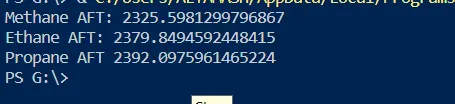
Conclusion:-
All four objectives are met and AFT for constant-volume, pressure, variation with Hydrogen atoms and variation with Carbon atoms.
- For the case of AFT for constant-volume, we see maximum deviation between the Python code logic and Cantera calculation. As Cantera uses the Gibbs Free Energy Minimization Technique to calculate the AFT which calculates the temperature upto the point where the Gibbs free energy is minimum. Where as this logic is not implied in Python code and it uses the formula for AFT for constant-volume.
- For FT constant-pressure process the maximum heat loss is multiplied by the heat loss factor. This factor ranges from 0 to 1. For the heat loss factor of 0, that is there is no heat loss the flame temperature is the AFT and thats why the value of Temperature for 0 heat loss factor is the highest. As the heat loss factor value is increased gradually to 1 the Flame temperature keeps falling down, at heat loss factor of 1 the flame temperature equals to 250 K.
- AFT variation with Hydrogen atoms, the combustion reaction is stoichiometric. For Ethyne(alkyne) the AFT at constant-pressure is the highest for comparing with the Ethene and Ethane.Ethyne>Ethene>Ethane or Alkane
- AFT variation with Carbon atoms, the combustion reaction is stoichiometric. The AFT for Propane (C3H8) so the AFT increases as the number of Carbon atoms increases. The AFT in our case is
Methane - AFT variation with Carbon atoms, the combustion reaction is stoichiometric. The AFT for Propane (C3H8) so the AFT increases as the number of Carbon atoms increases. The AFT in our case is