Week 3 - External flow simulation over an Ahmed body.
Aim : to simulate the external flow over Ahmed body and also calculate the aerodynamic forces over the body.
Q1. Describe Ahmed's body and its importance?
1. Ahmed Body.
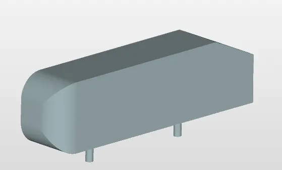
The Ahmed body is a generic car body (a simplified vehicle model). The airflow around the Ahmed body captures the essential flow features around an automobile and was first defined and characterized in the experimental work of Ahmed. Although it has a very simple shape, Ahmed body allows us to capture characteristic features that are relevant to bodies in the automobile industry.
This model is also used to describe the turbulent flow field around a car-like geometry. Once the numerical model in validated, it is used to design new models of the car. with the help of ahmed body a lot different studies eperimental as well as numerical cases are studied and confirmed , the effects of the drag and has captured deiiferent velocity profiles to design an optimum shape of the car.
Q2. Explain the reason for the negative pressure in the wake region.
When fluid velocity increases the pressure decrease. the wake region is formed due to adverse pressure (positive pressure) in the rear end causes the boundary layer to seperate out from the body the wall shear stress and velocity becomes zero and wake formation starts.the pressure in the wake region remains low as the flow seperates and a net pressure drag is produced. due to production of the pressure drag being produced from the flow seperation , the pressure in the wake region is low.
Q3. Explain the significance of the point of separation
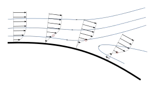
the boundary layer seperates when it has travelled far enough in an adverse pressure gradient that the speed of the boundary layer relative to the surface has stopped and reverse direction. at this point the flow seperates from the surface and form eddies and vortices.
the effects of the boundary layer seperation is regular shedding vortices known as von karman vortex street. vortices shed from the bluff body downstream surface of a structure at a frequency depending on the speed of the flow.another exampl of seperation is in the airfoils , the pressure field modification results in an increase in pressure drag, and if severe it also results in the stall and loss of lift.
Formulae Required : 1. reynolds number = density*U*linear characteristcs / µ
2. to calculate the first layer thickness
y+ = density*Utaw*▲y / µ
3.to calculate the Utaw :
Utow = √tow wall / density
4. to calculate tow wall :
tow wall = 0.5*Cf*density*U^2
5. to calculate the Cf value :
Cf = 0.0058*Re^-0.2
procedure for the simulation : 1. download the ahmed body from the provided link.
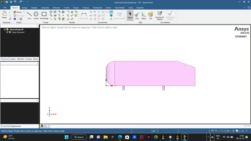
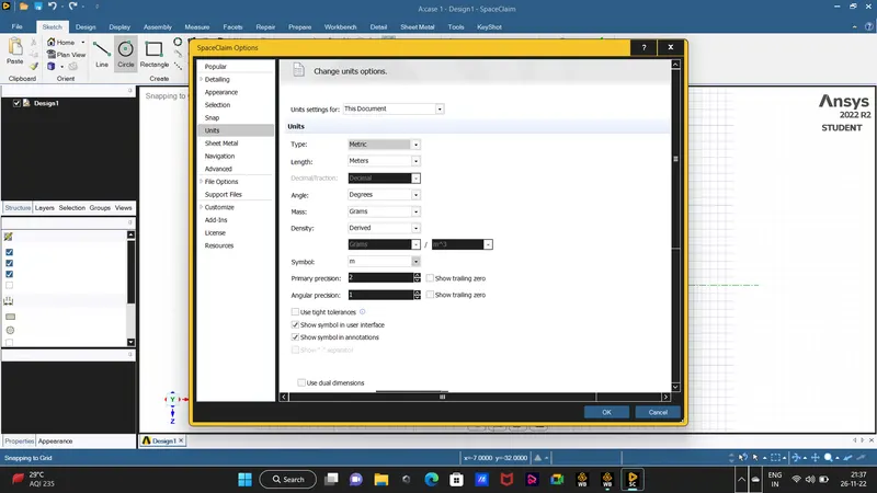
2. change the unit from millimeters to meter in the space claim before preparing the wind tunnnel. go to
files > spaceclaim options > units > change the units.
3. as we want to do the external simulation of the ahmed body we will enclose the ahmed body by using the enclose by using the enclosure in the space claim.
prepare > enclosure > select the ahmed body > switch off the symmetric option > enter the lenght for the winf tunnel.
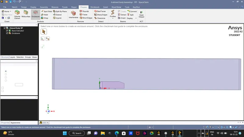 we will also create another wind tunnel inside the bigger wind tunnel because we have to capture the wake behind the ahmed body .
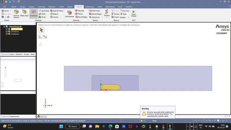 and this is how our geometry looks. the outer wind tunnel captures the geometry with the inner wind tunnel and the inner wind tunnel captures the body geometry.
4. we see that the ahmed body with the wind tunnel is symmetry so it is okay to split the model in half as it will also reduce the number of cell elemnts when we will refine the mesh.
to split the body go to : design > split body > select the outer wind tunnel body that you want to subtract the part > select the remove option > click the green arrow.
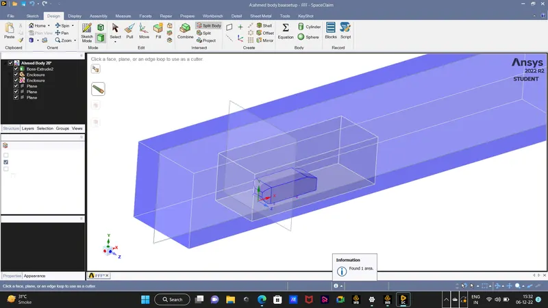 we will repeat the same steps for the inner wind tunnel and for the ahmed body.
5. as we split the body we also see the intersection of the hatches that causes the mesh to overlap and the mesh will not be good. so to clear this problem go to
prepare > interfernce > and select ok. > you will recieve message of the iterference problem is solved
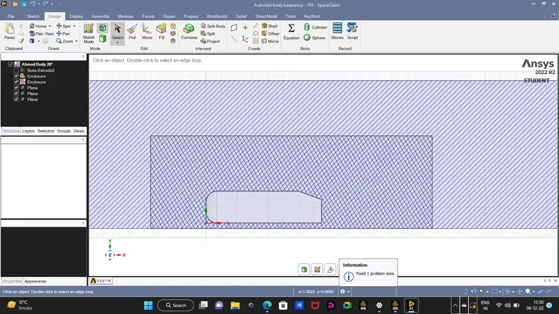 here we can see the hatches in the inner wind tunnel in two directions.
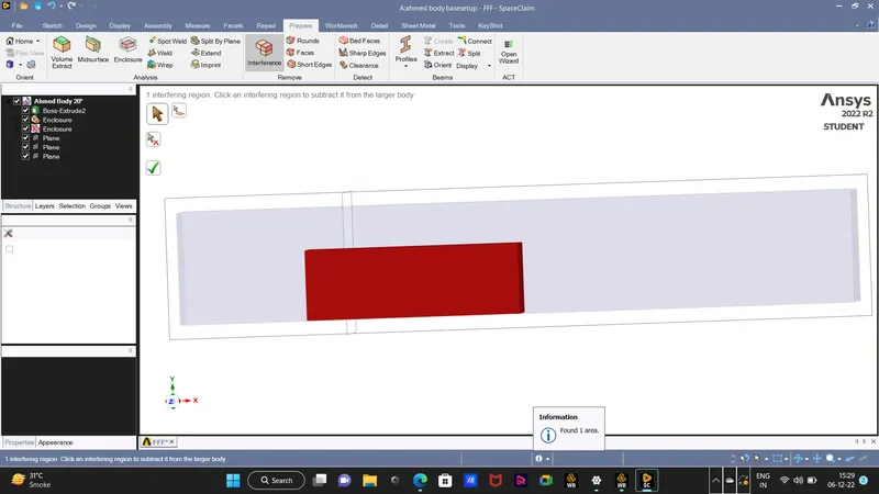 solving the interference .
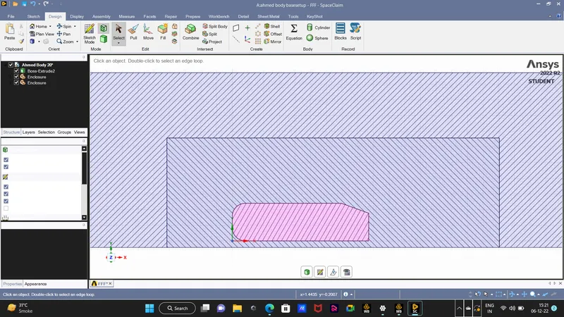 from the first snap we can see that the hatches in the inner wall are solved and the hatches are in one direction.
6. Mesh Setup :
naming the boundaries
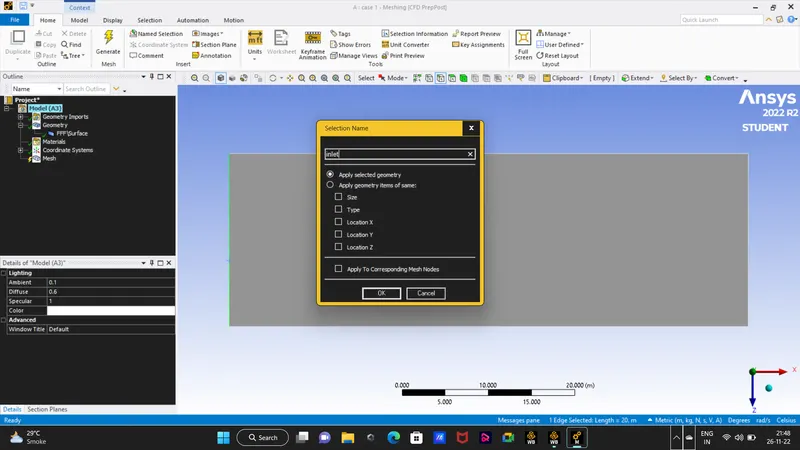
first we will go with the base mesh setup. that will be a coarse mesh but those mesh will not give a proper results.
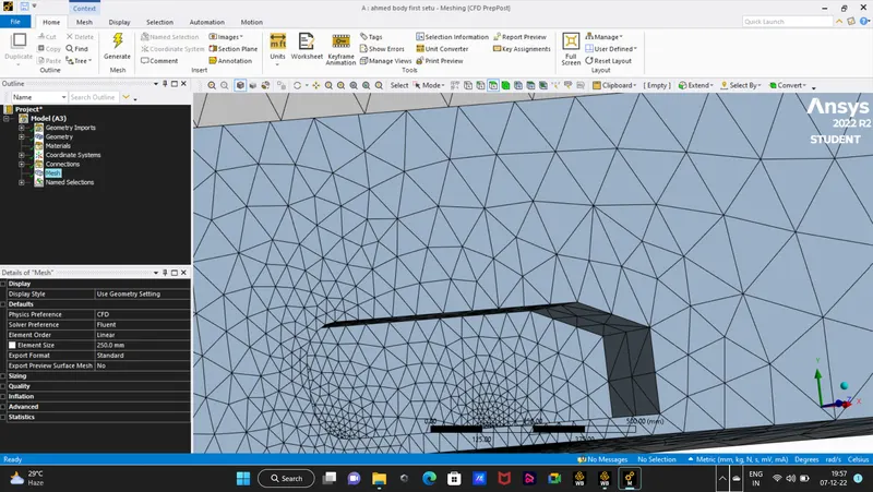
Refine Mesh :
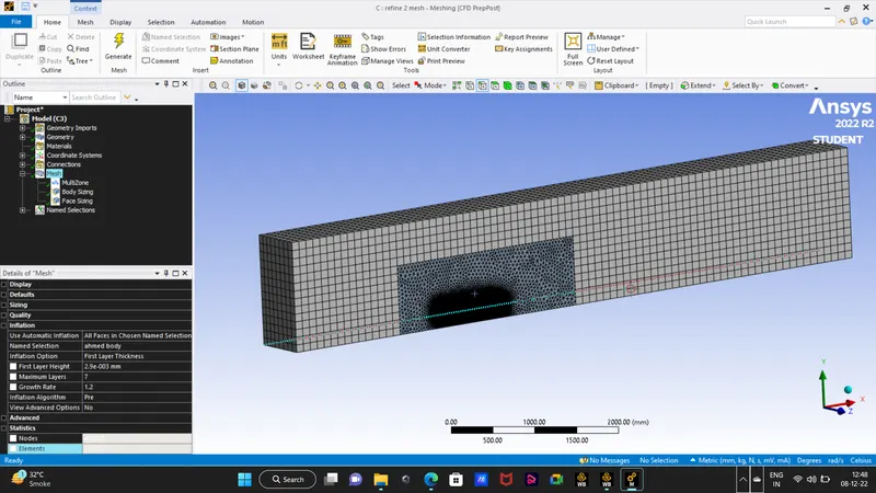
we will start with meshing the outer wind tunnel with the mutizone method and will create a hexahedral mesh. whenever the geometry is simple like our with straight lines like box we can go with the hexahedral mesh as they have the best quality to provide.to generte this mesh go to
mesh > insert > method > choose the outer wind tunnel body by selecting the ctrl+B > provide the mesh size > generate mesh.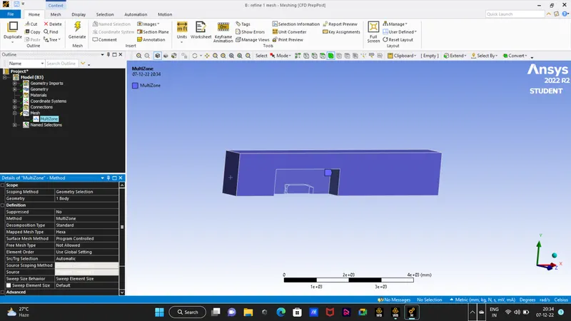
for the inner wind tunnel that will capture the wake behind the body we will refine the wall with sizing method
mesh > insert > sizing > select the inner wind tunnel body > enter the elemnt size for the body > generate mesh.
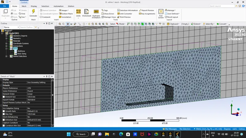
we will also refine the mesh on the ahmed body so that the mesh adopts the geometry properly. and also we will create inflation layers so that we can capture the boundary layer effects and also capture the velocity and other fluid parameters near the wall here comesh the y+ value as disscused in above topic.
to create the inflation layer > apply the named selection > select the ahmed body name > chose the First Layer Thickness > enter number of layers > enter the first cell height > generate.
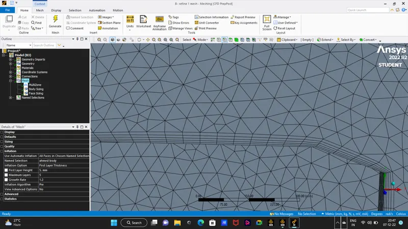
we will run the simulation for differnt mesh lenghts for the outer,inner, ahmed body , and also we will check the effects of the y+ value and also change the number of layers.
6. Fluent Setup :
for this project we will use
time : steady , type : density based , velocity formulation : absolute.
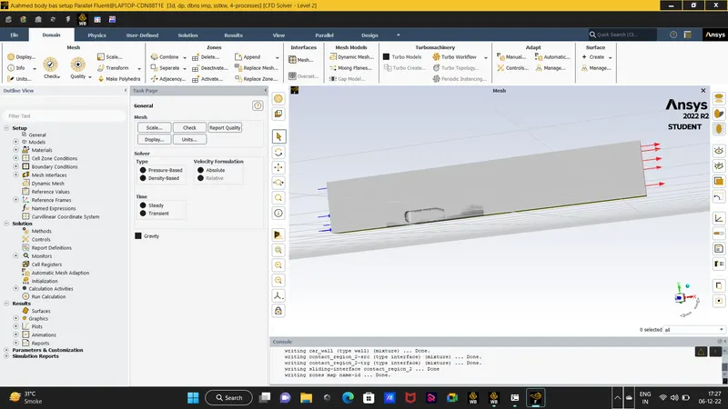
as the flow will be turbulent we will select the turbulence model, we will select the K-epsilon model, standardwall function.
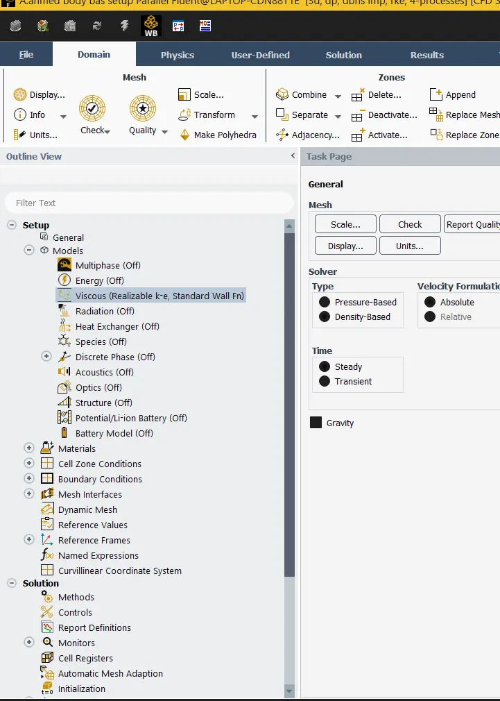 in cases where the fluid interacts with the solid countur the best choice will be k-omega as they are good for solving the flow near the wall.
entering the inlet velocity for 25 m/s
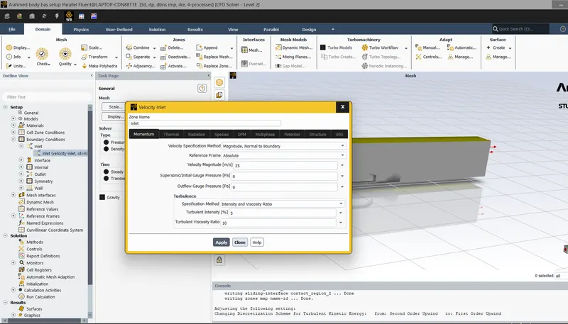
for the outlet the boundary conditions are set too pressure outlet for walls to symmtery.
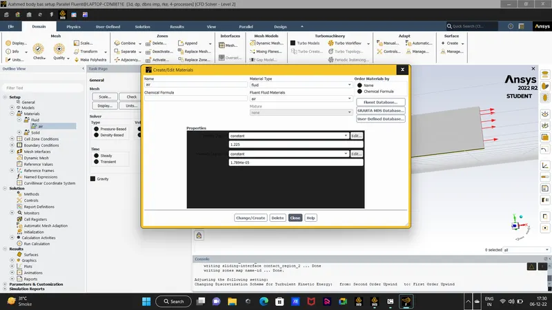
for the material properties we will keep as it is
materal type air , density = 1.225 kg/m^3 , viscosity = 1.789e-5 kg/ms
we also want to monitor the drag coefficient and lift coefficient we will create reports for that
solution > reports > force reports > drag and lift > lift coefficients > plot.
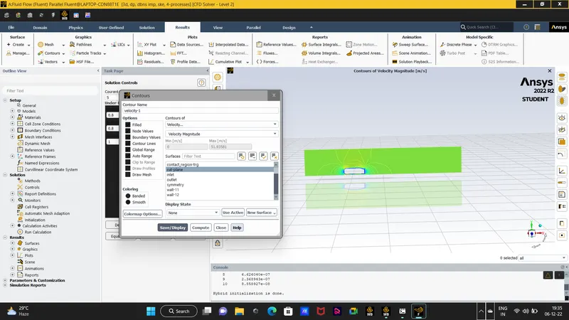
create countors for the velocity and pressure. but to first we have to do the initialization. we will use the hybrid initialization and then we will create the velocity and pressure countors.
results > countors > new > velocity and pressure > filled > dispaly and compute.
to make sure the drag and lift are plotted properly we will input the reference value and compute it from the ahmed body
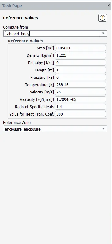
as we have already did the initialization with the hybrid selection we will just run the simulation and yield the result in the post process.
Expected Result :
tabular column : for mesh
outer wind inner wind ahmed body number of elements Cd Cl drag erorr %
tunnel tunnel
60 35 15 327521 0.36 0.450 11.2
80 40 15 290345 0.38 0.312 15.1
100 45 15 412098 0.42 0.40 27.2
120 50 15 70175 0.45 0.36 36.3
tabular coloumn : for y+
Y+ first cell total thickness number of layers
thickness
60 0.87mm 34.43mm 12
100 1.43mm 37.12mm 10
200 2.9mm 37.21mm 7
300 5mm 37.20mm 5
1. result for outer wall = 120 , inner wall = 50 , ahmed body = 15
y+ = 300
this first mesh was a basic mesh from this mesh lenght we calculated the y+ value and then we further adjusted the y+ value and the other mesh lenghts
mesh image
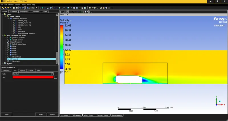 velocity result
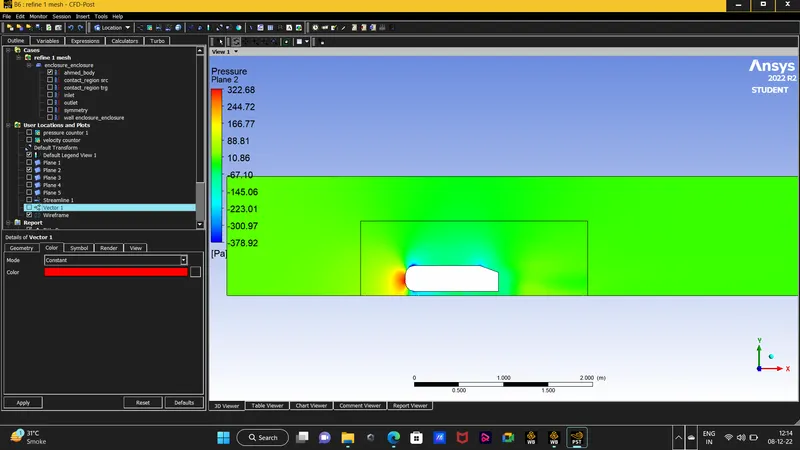 pressure result
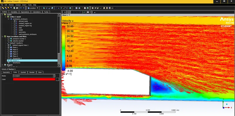 velocity vector
The result of coeefficients of drag and lift are Cd = 0.45 and Cl = 0.36
2. outer wall = 100 , inner wall = 45 , ahmed body = 15
y+ = 200
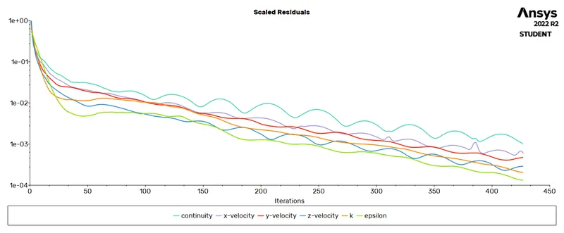
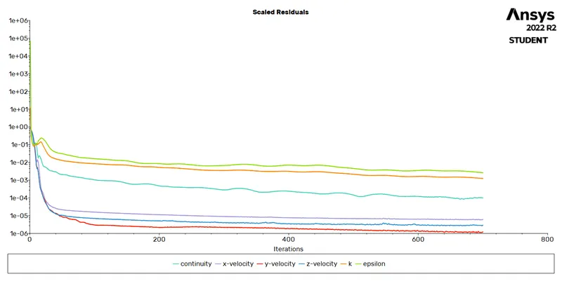 scaled residual
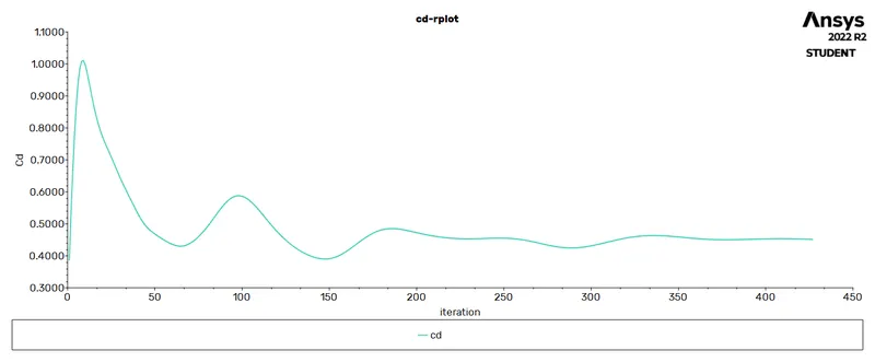
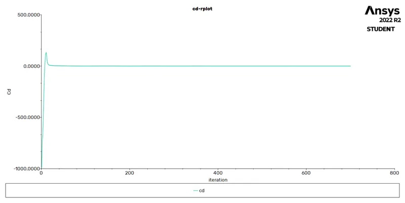 drag plot
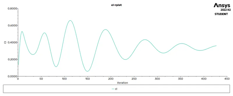
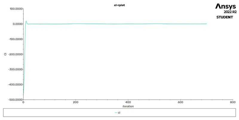 lift plot
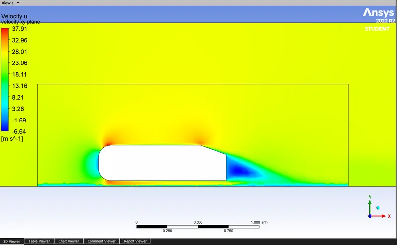 velocity result
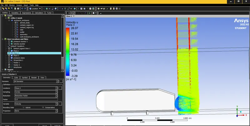 from this image we can see that the wake region is quite captured properly as we cn see recircualted fluid particles.
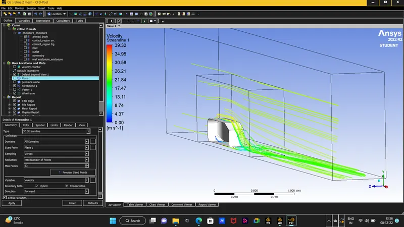
The result of coeefficients of drag and lift are Cd = 0.42 and Cl = 0.40
3. outer wall = 80 , inner wall = 40 , ahmed body = 15
y+ = 100
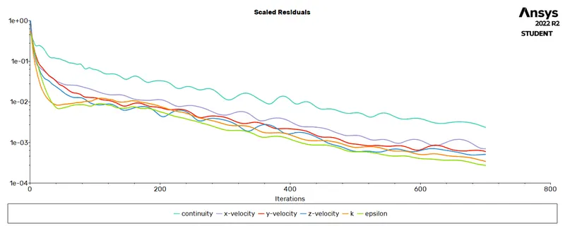 scaled residual
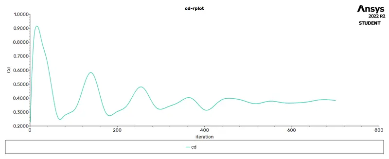 drag plot
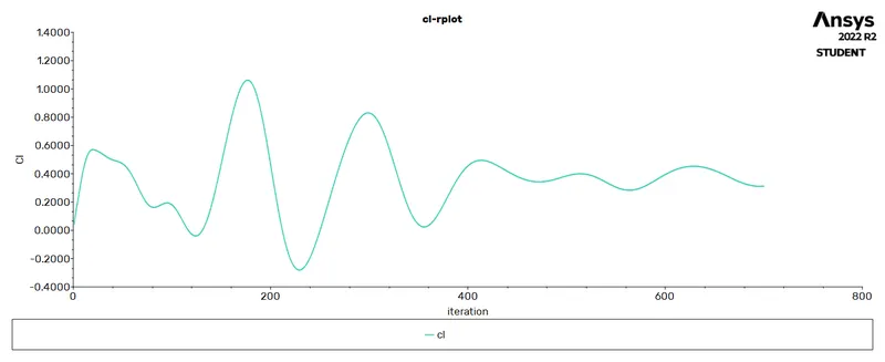 lift plot
velocity result 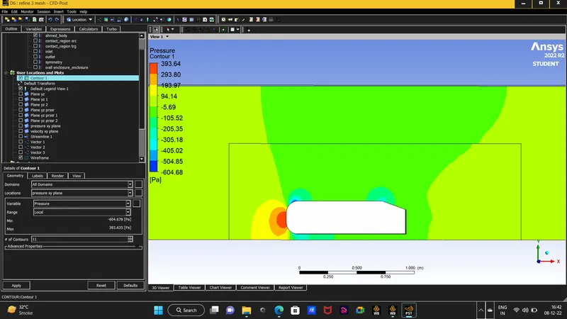 pressure contor
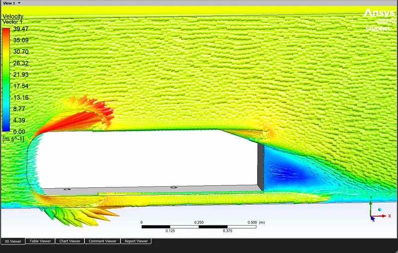 vector result
The result of coeefficients of drag and lift are Cd = 0.38 and Cl = 0.31
4. outer wall = 60 , inner wall = 35 , ahmed body = 15
y+ = 60
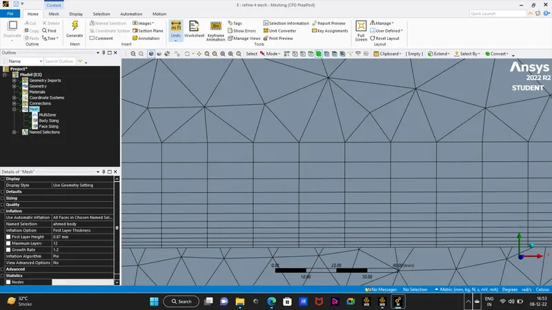 mesh result
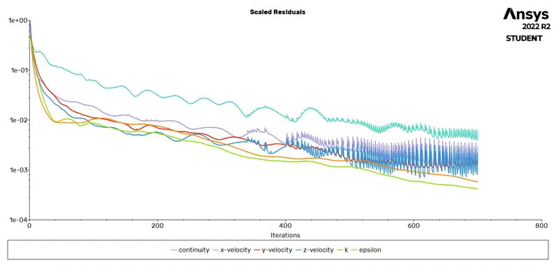 scaled residual
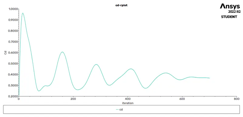 drag plot
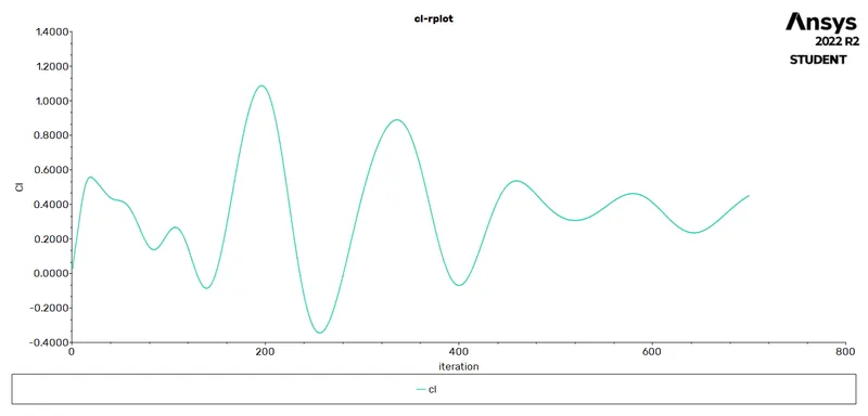 lift plot
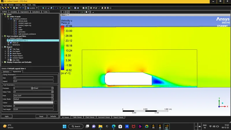 velocity result
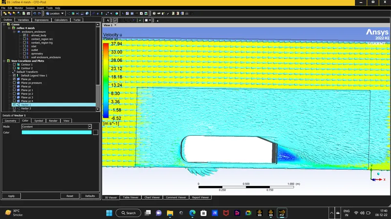
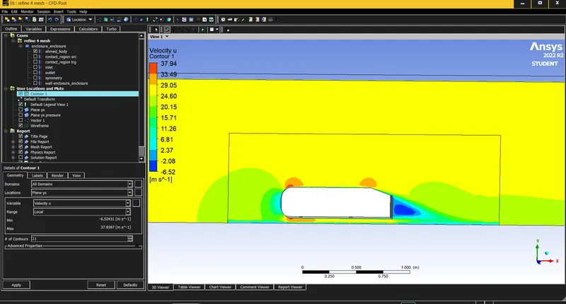 velocity contour
The result of coeefficients of drag and lift are Cd = 0.36 and Cl = 0.45
Grid Independence Test : as we know from the previous challenges that refining the mesh lenght will inrease the accuracy of the result but if the flow is turbulent there are effets of the boundary layer we learned about the concept of y+. adjusting the first layer cell height we saw the result getting accurate.the first cell height is important to capture the effects of fluid near the solid surface and we also conclued that from our smulation.
we run the simulation for different mesh lenghts and y+ values which from 300 to 60 values of the y+ we saw that the result for the darg over the ahmed body get accurate and closer to the estimated value of 0.33 for the y+ value of 60 the drag error is 11.2% while for the value of y+ of 300 the drag error is 36.3%. as we know that refining the mesh will increse the computational time but will give the accurate result the result for the drag for the y+ = 80 is 0.38 which is also acceptable but making the mesh more coarse will make the result more inaccurate which is not good. thus we can conclude that the simulation gave good result value for the value of 60 and 80 of y+ and also show promosing values.
Conclusion : experimental data did on the ahmed body has set a benchmark for doing the numerical simulation and designing the automobile for better fuel and drag efficiency.also learned about the different parameter to yield a proper and accurate result for the turbulent flows which has the effects on the solid boundary. inflation layers is very efficient to make a adaptive mesh around the body without increasing the number of elements drastically and also learned about the y+ value and how this factor also varies the result.