Week 2 - Flow over a Cylinder.

Aim : To construct a 2-D structure and simulate the flow over a circular cylinder for steady and transient state and explain the phenomena of Von Karman Vortex Street.

Requirement : 1. dimensions for creating the circular cylinder structure

diameter of circular cylinder (d) = 2m.

distance of inlet from the cylinder = 10*d.

distance of outlet from the cylinder = 20*d.

upper and below symmetry from the cylinder = 5*d.

Theory : VORTEX SHEDDING is an oscillating flow that takes place when a fluid flows past a bluff body at a certain velocities, depending on the size and shape of the body.in this flow vortices are created at the back of the body and detach periodically from either side of the body forming a Von Karman Street. the fluid flow past the object creates alteranating low pressure vortices on the downstream side of the object.Karman Vortex Street is a repeating pattern of swirling vortices caused by the process known as vortex shedding explained above which is responsible for unsteady seperation of flow of a fluid around the blunt body. it is named after the engineer anf fluid dynamicist Theodore von Karman and is responsible for 'singing' of suspended telephone or power lines or vibration of car antennas at certain speeds.a vortex street will form only at a certain range of flow velocities ,specified by a range of Reynolds Number(Re),typically above a limitting Re value of about 90.The frequency of vortex shedding can be dettermined by Strouhal Number (St). the strouhal number is dimensionless quantity that describes oscillating flow mechanisms.

St = Fd l/u

where, Fd = frequency of vortex shedding

l = linear dimension (diameter of cylinder or chord of airfoil)

u = flow velocity

we will compute the strouhal number by plotting the velocity at vortex point and then performing the Fast Fourier Transform in Fluent.Fast Fourier Transform (FFT) is done mainly to convert a sequence of signals in time domain to it frequency domain.

Procedure : 1. in this challenge we will create the geometry of the circular cylinder in the spaceclaim rather than downloading the model. to create the geometry first drag the fluent option in the working window and open the spaceclaim gui.

2.in the spaceclaim geometry change the measurement option from millimeters to meters. to do this go to file>spaceclaim option>units.

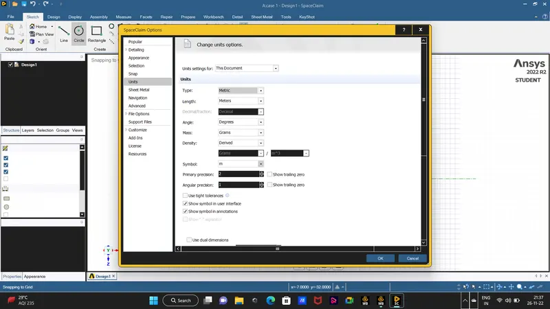after changing the units change the view to y-axis and by using the circle option in the design section draw a circle of 2m .then draw the surface with the help of the given dimensions.

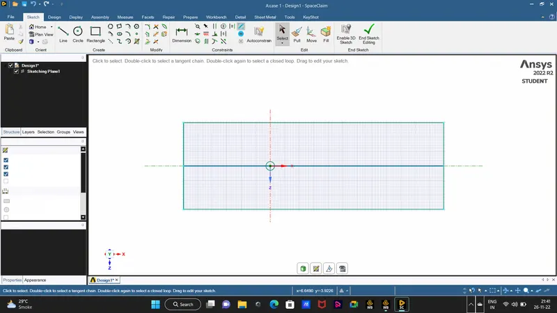this is how the geometry will look like.

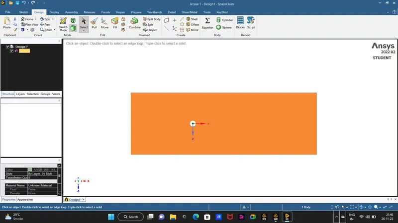
2. the geometry is just a sketch to compute the further process we need to convert the sketch to a surface.to do that we will use the pull option. got to design>pull> if the surface changes to orange colour than the surface is changed.now we will delete the circular part to do that go to design > Select > select the cylinder edges > delete the surface. and also delete the curves those are generated for creaton of the geometry.

3.MESHING

now we will start the surface to mesh. open the meshing gui there first we will see that the mesh is already generated in quadrilateral dominance.

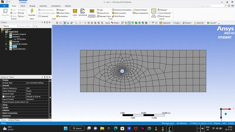to change the mesh elements to triangles go to insert method> geometry selection : select the surface body > apply > method : quad dominant change to triangles > generate the mesh. 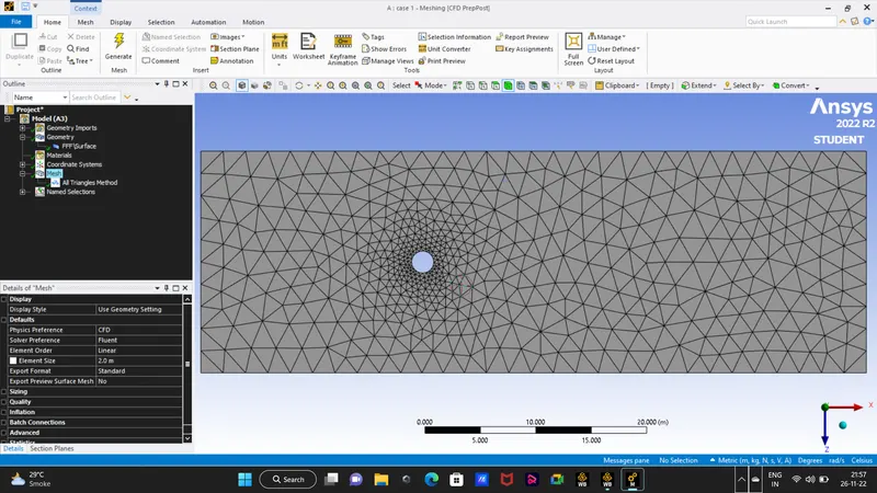as for our study this coarse mesh will not give proper results we will change the mesh size from default 2.0 m to 0.25 this finer mesh has provided the proper results

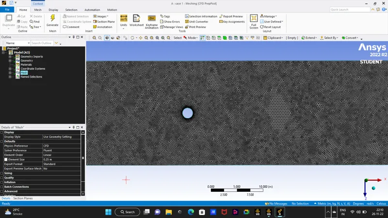
as our main corcern of computation is the surface closer to the cylinder we will make sure that the mesh in that region is very clean and clear so to make sure that we will also add inflation layers. infkation layers are also called adaptive body mesh, as the mesh adapt the geometry of the model very perfectly. to do that right click on the mesh > inflation layers > 1 select the body > select the boundary where you want the infaltion layer i.e the cylinder edges > inflation option : first layer thickness > first layer height : 5e-3 > maximum layers : 6 > generate mesh .

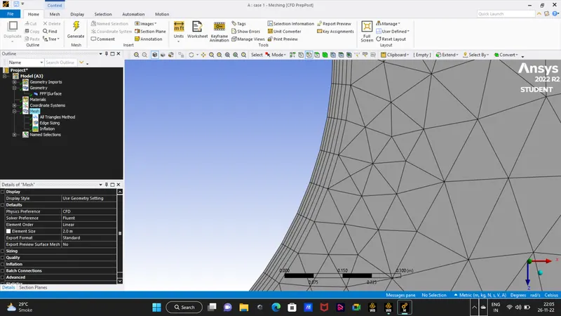here we can see that we have generated the 6 inflation layers of height 5e-3 from the surface and that grows at the rate of 1.2 and also name the boundaries of the surface

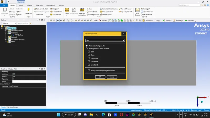here we are completed everything with the meshing and now we will proceed with the phyics setup and post proess.

4. open the fluent window and perfrom a mesh check for physics of the model we will select pressure based,absolute and for state we will select steady and transient both for our first case.

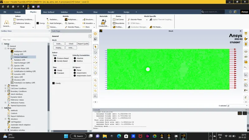
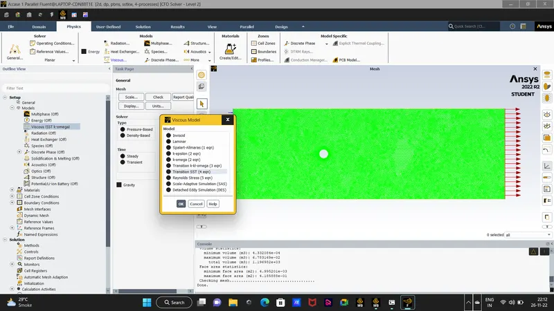
for the viscous model we will select the laminar option

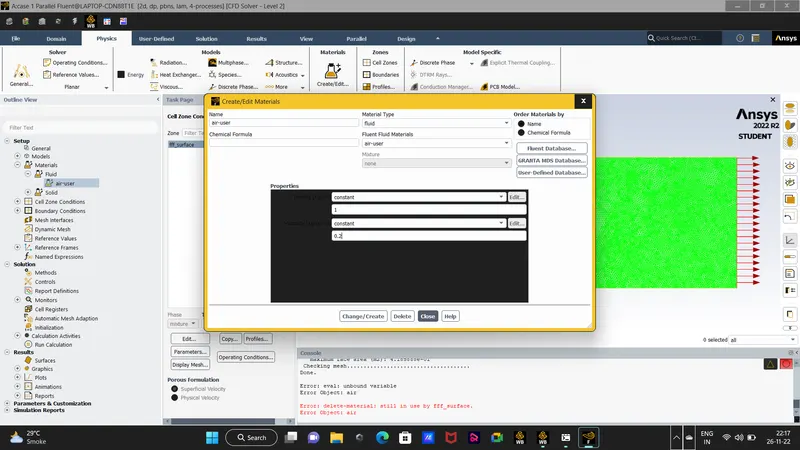
for our materail will create user material by selecting air in the fluent database and setting the density as 1 and the viscosity as 0.02 for reynolds number of 100

as the material selection is complete we will go and initiate the boundary conditions :

for the inlet we used the velocity inlet condition and the velocity of the inlet flow is set to 1m/s

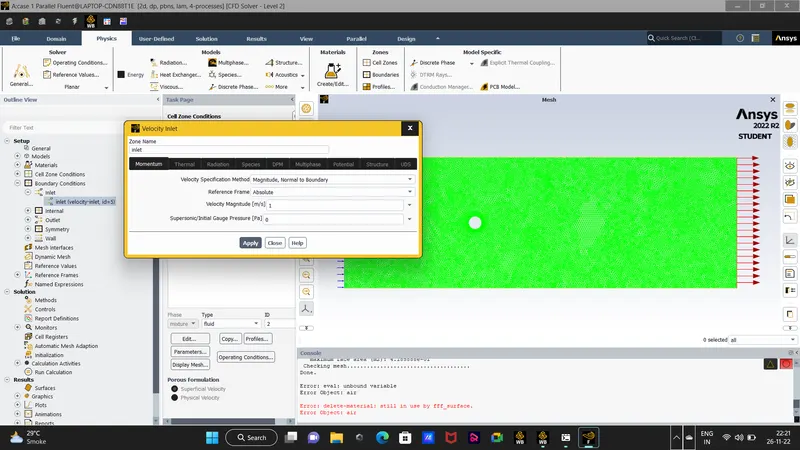
for walls i.e the cylinder walls boundary condition is set by fluent and here we will also select the No Slip condition for our first layer of the inflaton velocity to be 0

for the outlet the pressure outlet condition

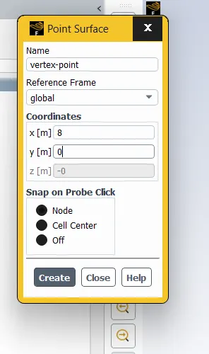
as the bpundary condition is set we also wants to monitor some variables at the solution gets converged so do that first we will create a point at a distance of 4*d from the cylnder at the downwash of the body to calculate the vertex velocity . to do that go the results > surface > create > point > enter the x(m) = 8 and y(m) = 0 name as vertex-point > create

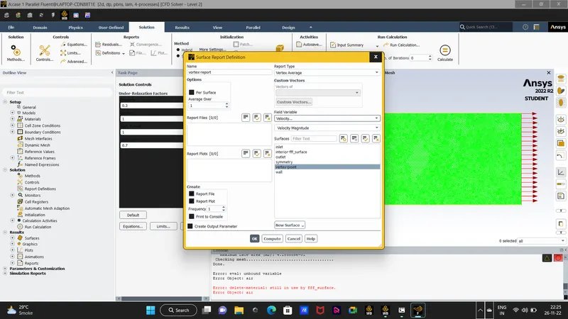
now we will difine report at the created vertex point go to solving > definitions > new > surface report > area weighted vortex average > of velocity > at the vortex-point > report file and plot > ok.

same way we will create the report for the coefficeints of lift and drag.

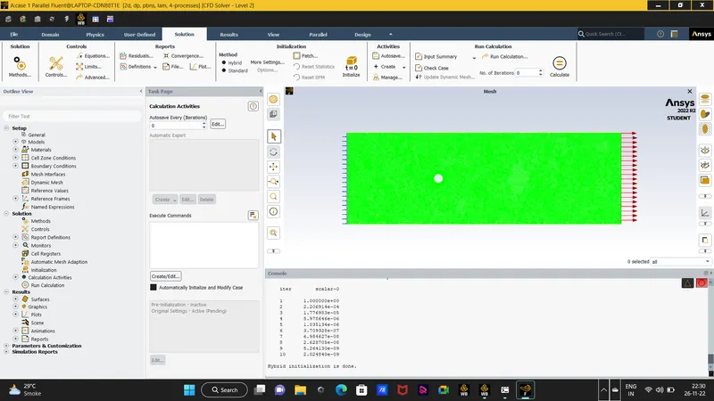
we will also create counour plots for the velocity and pressure but for that first we ahve to initialize the solution so that those initial conditions will be used to compute the contour plots withe solution getting solved at the same time. to create the contour initiate the hybrid initialization.

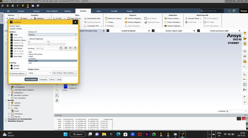
then go to results > graphics > contours > new > name as velocity > select the filled option > contour of velocity > select all the surfaces > save/display > compute.

as the solution changes as the number of iteration we will compute animation of the solution for each 10 iteration solved. to do that go to

solution > activities > create > solution animation > name as velocity-animation or otherwise the name will conflict with the contour name > store type = 10 > select the velocity > ok.

as we are done with setting up the physics naming the material everything and we have already initialized the solution for the steady solver we will compute for 500 iteration and for the transient solver we will initialse time step size as 0.1 s and number of steps as 500 for initially but for the transient state we have to run the simulation for a pretty long time still the solution dont gets to a steady state.for the steady solver the solution will get converge around 500 to 800 iterations.but for the steady state condition we will not be able to compute the strouhal number becase the strouhal number is the function of the time so the strouhal will be only compute for the transient state and for that purpose we will compute the transient state too.

5. the strouhal number for the transient state will be compute after the solution got computed, becase to compute the strouhal number we need the area weighted average vortex plot of velocity to then we will go to the reuslts > FFT > for the y-axis we will select the magnitude and for the x-axis we will select the strouhal number > input file : here we will input the area weighted average vortex plot of velocity > compute the plot .

6. do the procss for the case 1 and case 2 and show the expected results.

expected results :

CASE 1 : Simulate the flow with the steady and unsteady case and calculate the Strouhal Number for Re= 100.

(a). for Steady state case : for the cases the reynolds number is set to 100 in the fluent we will control the reynold number by changing the viscosity of the air. the steady state is sufficient to plot the lift and drag cofficients plot but to compute the stouhal number we need the transient state as the strouhal number changes with time.

convergence plots for the steady case :

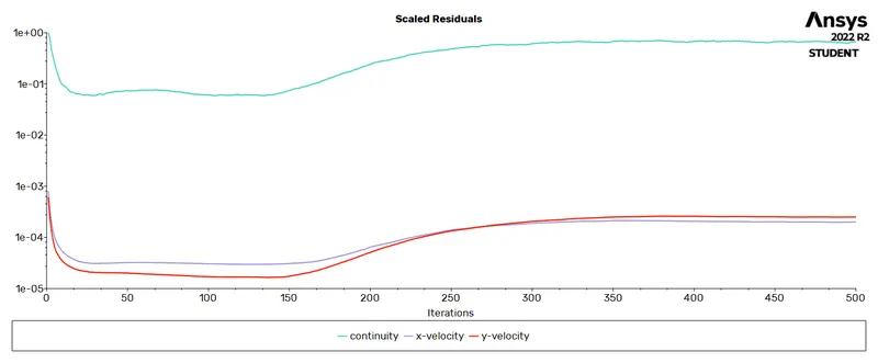plot for the residual, the residual converged at e-4 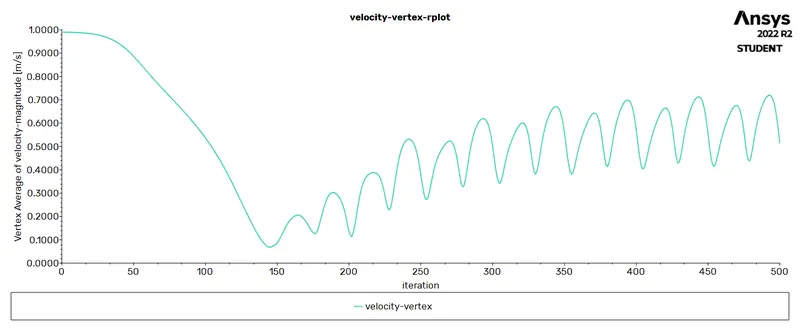vertex average velocity magnitude plot

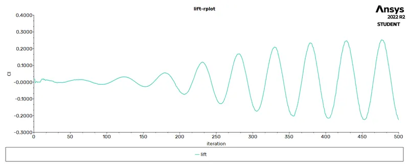coefficicent of lift plot

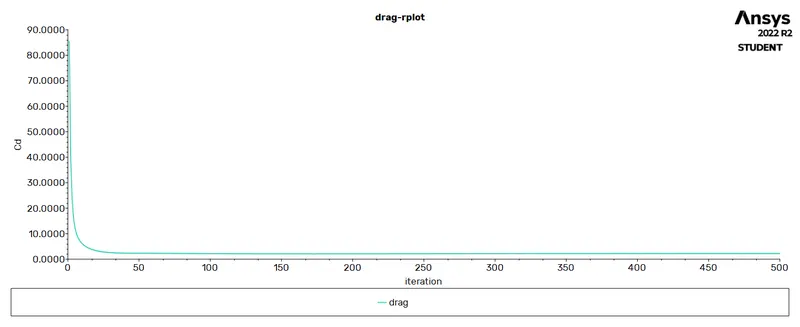coefficient of drag plot

the plots above for the steady state shows the same repeating pattern from 300 iterations and hence we can conclude that the solution has got converged.

the value of coefficients of lift and drag is computed and is equal to Cl = -0.071 and Cd = 1.358

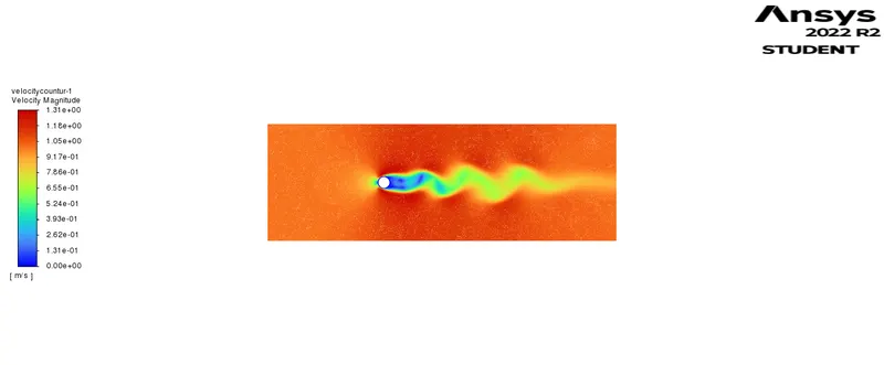
(b). Transient state :

convergence plot :

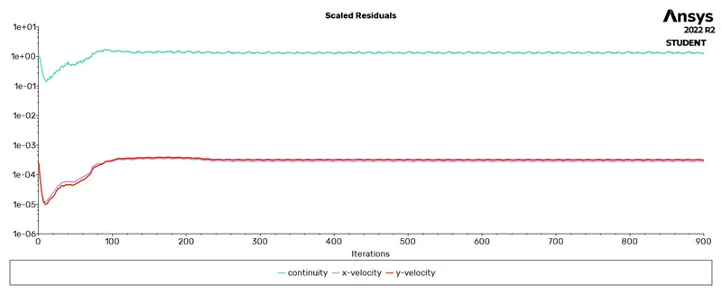
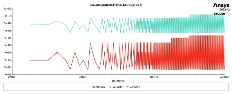scaled residual plot

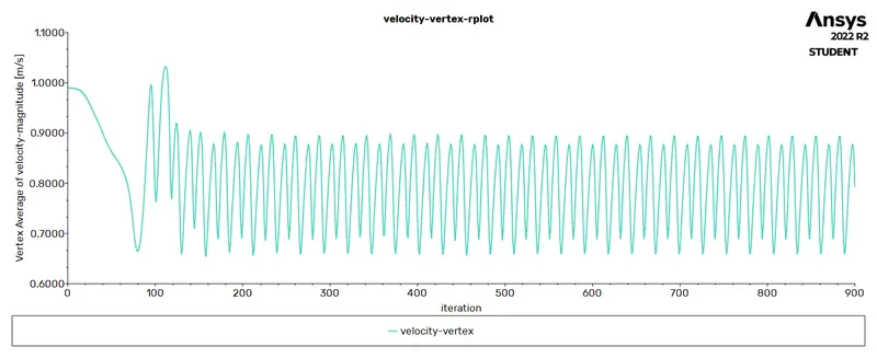
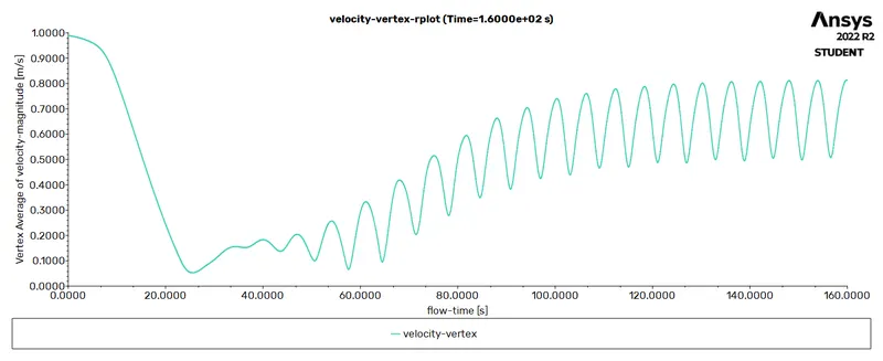velocity-vertex plot

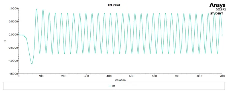
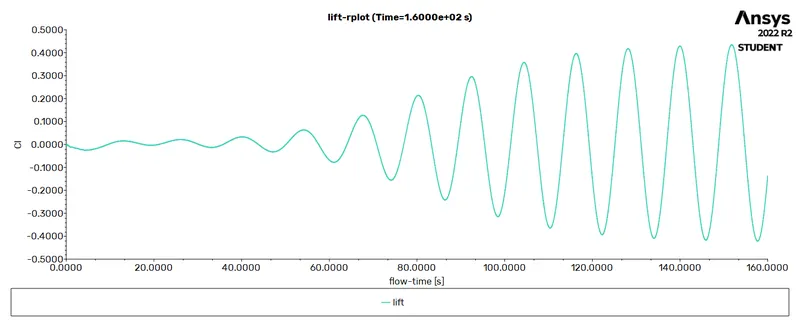lift plot

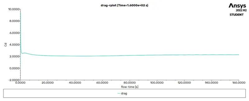from the Cl, Cd , velocity-vertex report we can say that the solution shows a repeating pattern after 100 seconds so we can say that the solution is converged.in the transient type states the perfect flow simulation as it takes place in the real world.

the value of of the coefficients of lift and drag computed are Cl = -0.249 and Cd = 1.394 the value of the cl is negative beacuse the lift plot stops at the growing resion from downwards and so the computed value that ansys provide is in negative.

the computed values when compared to the reference paper values for 100 reynolds number that is for Cd = 1.335 and Cl = 1.792 when compared to these values the difference in the Cd value is of 0.059 that is very small and we can say that the error is acceptable and our computation values are valid.

as we stated that the strouhal number is an time dependant value so we plotted the graph for the strohal number

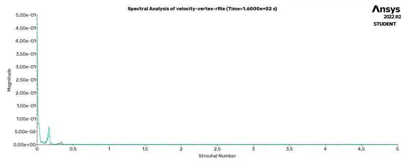the graph plotted is strouhal number V/s

magnitude the value of the strouhal numebr obtained from the graph is 0.167

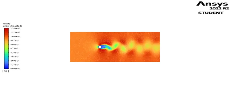
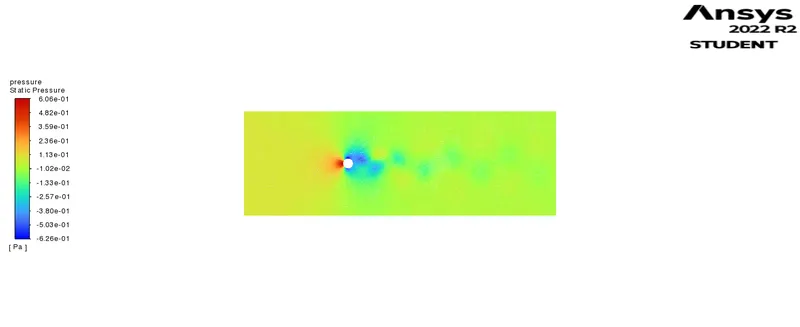
Case Cl value Cd value Strouhal Number

1.steady state -0.0071 1.358 _____

Re = 100

2.transient state -0.249 1.394 0.167

Re = 100

3.values from the 0.1792 1.335 0.156

refernece paper https://www.sciencedirect.com/science/article/pii/S0307904X08000243

Case 2 : calculate the coefficients of drag and lift for Re of 10,1000,10000,100000 for steady state solver

for Re = 10

convergence plots

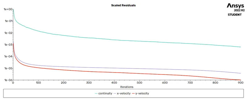
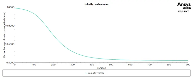
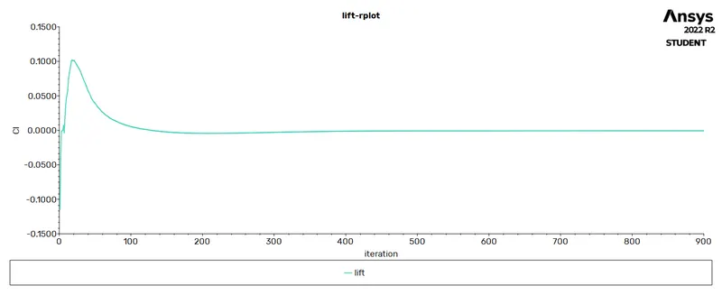
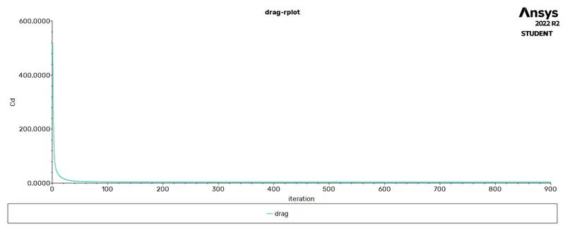
convergence plots for the cl,cd, velocity-vertex and scaled residual.here from the plots we can conclude that at reynlods number of 10 we dont see any wake as the flow is laminar and the flow seperation is very small as stated in the refrence paper that the speration or vortex shedding at the circular cylinder depends on the flow properties.

Re = 1000

convergence plots

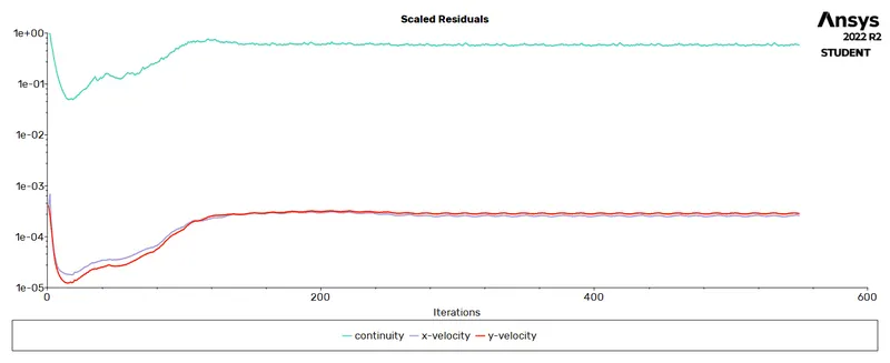
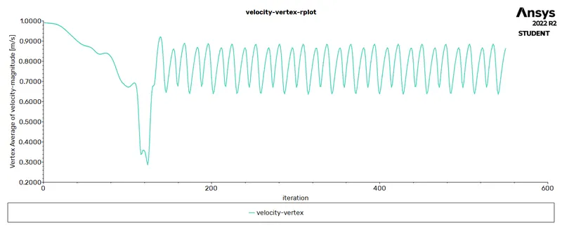
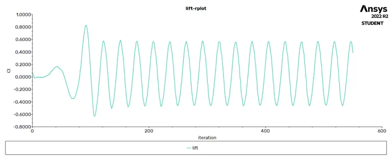
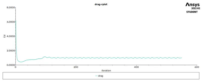
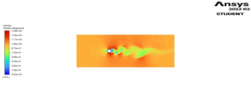the Cl,Cd, scaled residual, velocity-vertex plots are shown the simulation for these plots are run for 600 and for more iteration but the solution converges at 150 iterations as it shows same repeating pattern.from the plots of Re 100 and 1000 we can say that the vortex becomes more disfused as well as the frequency of the shedding also becomes very high.

Re = 10000

covergence plots

Re = 100000

convergence plots

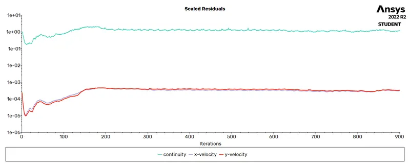
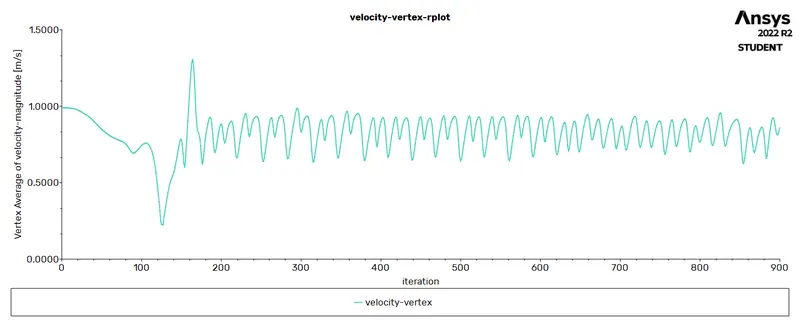
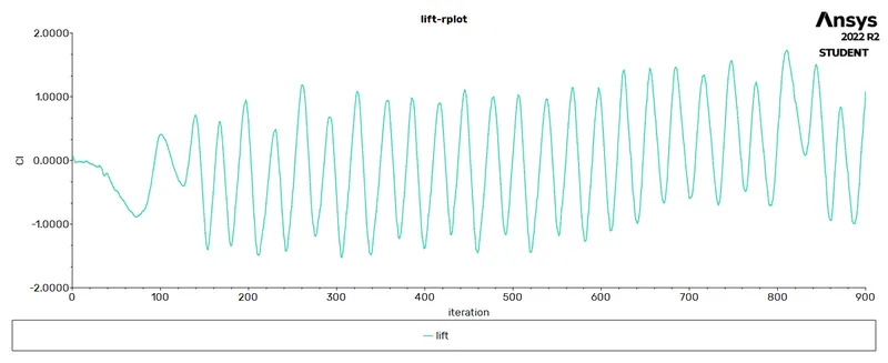
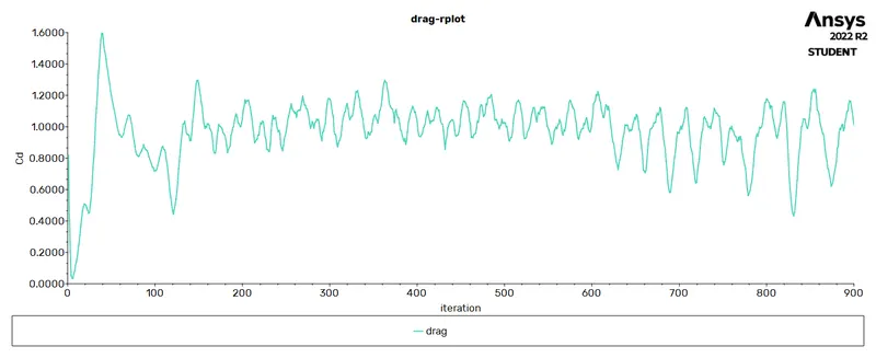
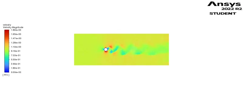
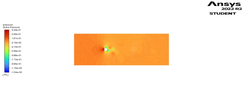
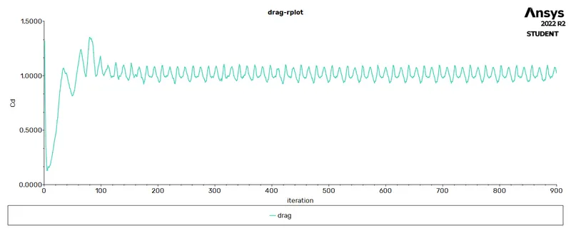
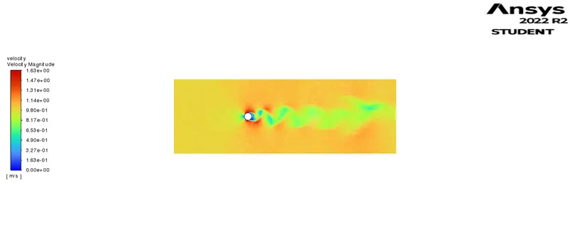
the convergence plots for the re 100000 is shown the drag and the lift drastically changes and the from the plots we can see that the lift and drag changes right from the very start even before the iteration reaches 100 the lift starts to change as well as the drag. the frequency of the vortex shedding also changes very early as compare to re of 100 and 1000 that means the downwash flow from the body seperates very quickly and the vortex shedding is very turbulent.

Conclusion : in this challnege we did computation of the flow over the circular cylinder for different Reynolds number and also see the phenomenon of the von karman vortex street. from the results computed we can say that the vortex shedding depends on the reynolds number or in other words the velocity of the flow, as we did the computation for reynolds number from 10 to 100000 we can say that as the reynold number increases the flow velocity increses that makes the flow to change from laminar to turbulent that makes the flow to seperate the cylinder more rigoursly and making the vortex shedding more diffused and the flow to be more turbulent on the downwash of the cylinder. and also the reynold number affects the lift and drag coefficients too as the reynolds number increses it makes the flow to be more turbulent that decreses the lift value and the pressure drag increases as becuase at high renolds number the dominant forces are the inertial forces that means the pressure drag will be high.