Week 5.1 - Mid term project - Solving the steady and unsteady 2D heat conduction problem

Aim : Solve the Steady ans Transient State for the 2-D Heat Conduction Equation with Implicit and Explicit schemes and implement the following Iterative Solvers for solving the Implicit Equation.

1. Jacobi Method
2. Gauss-Seidel Method
3. Successive Over Relaxation Method

Requirements : Boundary Conditions.

Top Boundary = 600 K

Bottom Boundary = 900 K

Left Boundary = 400 K

Right Boundary = 800 K

Tolerance = 1e-4

Theory : The Heat Conduction Equation is a Partial Differential Equation that describes how the distribution of heat evolves over time in spatial domain.Heat flows spontaneously from Higher temperature regions to Lower Temperature region.The Heat equation in three dimension the Temperature is the function of (x,y,z,t).

`(delT)/(delt) 1/alpha = (del^2T)/(delx^2)+ (del^2T)/(dely^2)+(del^2T)/(delz^2)`

is the equation for 3-D.Where `alpha` is the constant of Thermal Diffusivity of the material is the thermal conductivity divided by density and specific heat capacity at constant pressure. It measures the ability of a material to conduct thermal energy relative to its ability to store thermal energy. High diffusivity means heat transfers rapidly.

as to solve the 2-D heat equation,Temperature will be the function of (x,y,T) the equatiion will be

`(delT)/(delt) 1/alpha = (del^2T)/(delx^2)+ (del^2T)/(dely^2)`

Steady State equation will be solved only for the spatial term the time depenedent term of the equation will be zero.Therfore the equation will be ;

`(del^2T)/(delx^2)+ (del^2T)/(dely^2) = 0`

The Transient Equation for 2-D heat equation is given as :

`(delT)/(delt) = alpha (del^2T)/(delx^2)+ (del^2T)/(dely^2)`

The steady state equation is parabolic PDE therfore the we have to take the information from all the points to solve the equation,therefore the equation will be discretise with the Central Differencing Scheme,

`(del^2T)/(delx^2)+ (del^2T)/(dely^2) = 0` ----(1)

`(T_(i+1,j) - 2T_(i,j) + T_(i-1,j))/dx^2 + (T_(i,j+1) - 2T_(i,j) + T_(i,j-1))/dy^2` -----(CDS discretization)

Rearranging the equation and we get,

`T_p = 1/k[(T_l + T_r)/dx^2 + (T_t + T_b)/dy^2]`

where `k = (2*(dx^2 + dy^2))/(dx^2 + dy^2)`

`T_p = T_(i,j)`

`T_l = T(i-1,j)

`T_r = T_(i+1,j)`

`T_t = T_(i,j+1)`

`T_b = T_(i.j-1)`

`T_p = (term1 + term2)/k`

where term1 = `(T_l + T_r)/(dx^2)`

term2 = `(T_t + T_b)/(dy^2)`

• Code for 2-D Heat Conduction for the Steady State using the Iterative Methods :

%2-D Heat Condution Steady Code

clear all
close all
clc

%inputs
l = 1;                    %length of domain
nx = 10;                  %number of grid points along x 
ny = 10;                  %number of grid points along y
error = 9e9;
tol = 1e-4;               %Tolerance value

%creating 2-d mesh
x = linspace(0,l,nx);
y = linspace(0,l,ny);
dx = x(2) - x(1);
dy = y(2) - y(1);

k = 2*(dx^2 + dy^2)/(dx^2 * dy^2);        %term for computating the value

T = 300*ones(nx,ny);             %Inital guess for temperature

for i = 2:nx -1                  %Top and Bottom B.C
  T(1,i) = 600; 
  T(nx,i) = 900;
end  

for j = 2:ny -1                %Left and Right B.C
  T(j,1) = 400;
  T(j,nx) = 800;
end

%Corners nodes B.C
T(1,1) = (T(1,i) + T(j,1))/2;
T(nx,1) = (T(j,1) + T(nx,i))/2; 
T(nx,ny) = (T(nx,i) + T(j,nx))/2;
T(1,ny) = (T(1,i) + T(j,nx))/2;

Told = T;

printf('1.Jacobi\n2.Gauss Seidel\n3.SOR\n');
method = input('Select Iterative Method = ');

if(method == 1)           %Jacobi Iterative method
  tic;
  j_iter = 1;
  while(error > tol)
    for i = 2:nx-1
      for j = 2:nx-1
        term1 = (Told(i-1,j) + Told(i+1,j))/(dx^2);
        term2 = (Told(i,j+1) + Told(i,j-1))/(dy^2);
        T(i,j) = (term1 +term2)/k;
      end
    end
    error = max(max(abs(T - Told)));
    Told = T;
    j_iter = j_iter +1;
    sim_Time_jacobi = toc;
  end
  
  figure(1)
  colormap(jet);
  X = contourf(x,y,T);
  clabel(X);
  colorbar;
  xlabel('X');
  ylabel('Y');
  set(gca,'YDir','reverse');
  txt1 = sprintf('Number of Iterations for Steady Jacobi Method = %d',j_iter);
  txt2 = sprintf('Total Simulation Time for Jacobi = %f',sim_Time_jacobi);
  title({'2D Heat Conduction Steady State Profile for Jacobi Method';txt1;txt2});

end  

if(method == 2)           %Gauss Seidel Iterative Method
  tic;
  gs_iter = 1;
  while(error > tol)
    for i = 2:nx-1
      for j = 2:nx-1
        term1 = (T(i-1,j) + Told(i+1,j))/(dx^2);
        term2 = (Told(i,j+1) + T(i,j-1))/(dy^2);
        T(i,j) = (term1 +term2)/k;
      end
    end
    error = max(max(abs(T - Told)));
    Told = T;
    gs_iter = gs_iter +1;
    sim_Time_gs = toc;
  end
  
  figure(1)
  colormap(jet);
  X = contourf(x,y,T);
  colorbar;
  clabel(X);
  xlabel('X');
  ylabel('Y');
  set(gca,'YDir','reverse');
  txt1 = sprintf('Number of Iterations for Steady Gauss Seidel Method = %d',gs_iter);
  txt2 = sprintf('Total Simulation Time for Gauss Seidel = %f',sim_Time_gs);
  title({'2D Heat Conduction Steady State Profile for GS Method';txt1;txt2});

end  

if(method == 3)           %SUCCESSIVE OVER RELAXATION ITERATIVE METHOD
  omega = 1.3;            %relaxation factor
  
  tic;
  s_iter = 1;
  while(error > tol)
    for i = 2:nx-1
      for j = 2:nx-1
        term1 = (T(i-1,j) + Told(i+1,j))/(dx^2);
        term2 = (Told(i,j+1) + T(i,j-1))/(dy^2);
        T(i,j) = Told(i,j)*(1-omega) + omega*((term1 +term2)/k);
      end
    end
    error = max(max(abs(T - Told)));
    Told = T;
    s_iter = s_iter +1;
    sim_Time_sor = toc;
  end
  
  figure(1)
  colormap(jet);
  X = contourf(x,y,T);
  colorbar;
  clabel(X);
  xlabel('X');
  ylabel('Y');
  set(gca,'YDir','reverse');
  txt1 = sprintf('Number of Iterations for Steady SOR Method = %d',s_iter);
  txt2 = sprintf('Total Simulation Time for SOR = %f',sim_Time_sor);
  title({'2D Heat Conduction Steady State Profile for SOR Method';txt1;txt2});

end

• We start the code while initializing and declaring the inputs. l is the length of the domain in(m), the nx=ny=10 that is the number of grid points along x and y.
• We create a 2d mesh with the linspace function,then we calculate the dx and dy value for computation of the T(i,j).
• We will create the Boundary Conditions as stated with the Initial Conditions. The Code line T = 300*ones(nx,ny),creates the Inital condition for the temperature with 300 K for all the 10 grid points in x and along y.
• To assign the Boundary Conditions along Top and Bottom boundary, we used the 'for' loop and assigning the i = 2:nx-1, that will be i will be the range of 2 to 9.So the line after the for loop T(1,i) = 600, assigns the value 600 for the range of 1 row and the range of 2 to 9 will be in the y-direction that makes the Top Boundary.And similarly the for the Bottom Boundary T(nx,i) = 900, will assing the 900 to the last row and the range of 2 to 9 along the column.
• Similarly, the Left and Right Boundary is assigned.
• The corners elements of the Temperature profile will be calculated by taking the average of the adjacent nodes to that corner node.Then assinging the T value to Told.
• We also take an input from the user to select the appropriate the method to solve the code.
• To start the computation we will start the with the 'if' this helps to match the input from the user and check with the if condition.The (==) matches the values.According to the IF condition the code will run the respective part of the code.
• When the IF condition matches with the appropriate method the " tic " will start to record the computation time for the solver.To count the number of iterations it took to reach the convergence,and set it to 1.
• We will start with the convergence loop while(error > tol).Uptil the error is greater than the tolerance value the temperature value for the node value i and j will be calculated,and then the value of error is calculated.Then if the error value is reached to the tolerance the T value is updated to Told as well as the iteration value.
• And in the convergence loop record the time for the simulation for the method.
• Plot the contour value of T and also mention the iterations and simulation time for the respective method.

The formulas for the Itertive method for;

• Jacobi the value of T(i,j) is calculated from the old values of T to calculate the new iterative values.
• For Gauss-Seidel Method the value of T(i,j) is calculated with the updated value of the previous T,that is ;

`T_(i,j) = ((T_(i-1,j) + Told_(i+1,j))/dx^2) + ((T_(i,j-1) + Told_(i,j+1))/dx^2)`

• from the above the formula T(i-1,j) is the updated iterative value as for the (i,j) the T(i-1,j) and T(i,j-1) is already calculated and updated.
• For the SOR method we will select the relaxation factor to be 1.1 or 1.3 to be over-relaxed and the formula (dT/di) is calulated in the with the Gauss-Seidel Method.

Results for the Steady State code :

• Steady State Jacobi Method results

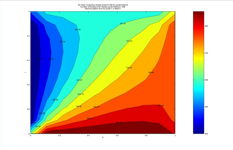
Number of Iterations for Jacobi = 208

Simualtion Time = 0.29 sec

• Steady State Gauss-Seidel Method results :

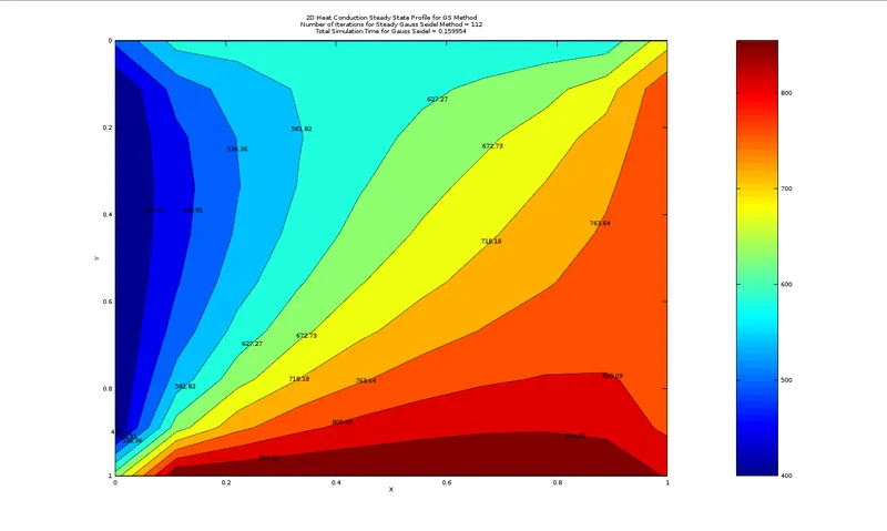
Number of Iterations for Gauss-Seidel = 112

Simualtion Time = 0.16 sec

• Steady State Successive Over Relaxation Method results :

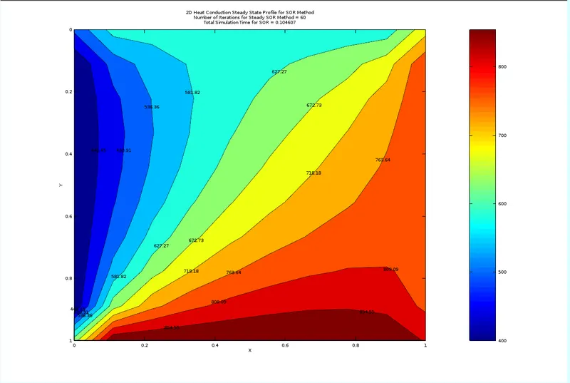
Number of Iterations for SOR = 60

Simualtion Time = 0.10 sec

• Transient State 2-D Heat Conduction Equation Explicitly :

`(delT)/(delt) = alpha (del^2T)/(delx^2)+ (del^2T)/(dely^2)` -----(2`

The above equation is solved for both Explicit and Implicit Methods.`(delT)/(delt) = alpha (del^2T)/(delx^2)+ (del^2T)/(dely^2)`

Explicit approach in the numerical analysis for obtaining numerical approximations to the solution of time-dependent ODE or PDE as in required for computer simulation for the physical process.

Explicit method calculates the future status of the system by taking the information from current state of the system at current time State.However, the time step is limited by the size of the numerical stability. Accordingly, this method is considered as conditionally stable, because if the time step is too large, there will be a significant numerical error. In explicit, the system contains only one unknown.

The time dependent term will be discretize the with backward differencing scheme.

`(T_p^(n+1) -T_p^n)/dt = alpha[(T_l-2T_p+T_r)^n/dx^2 + (T_t-2T_p+T_b)^n/dy^2]`

where n = old time value

and n+1 = new time value

Rearranging the terms in the equation we get;

`T_p^(n+1) = T_p^n + k1(T_l-2T_p+T_r)^n + k2(T_t-2T_p+T_b)^n`

where k1 = `alpha(dt)/dx^2` which is also Courant number along x

and k2 = `alpha(dt)/dy^2` Courant number along y

The Diffusion Stability for the 2-D heat conduction is given as

`alpha_x(dt)/dx^2 + alpha_y(dt)/dy^2 <= 0.5`

Simplifying the equation term1 = `Told_(i,j)`

term2 = `k1(T_l-2T_p+T_r)`

term3 = `k2(T_t-2T_p+T_b)`

`T_(i,j) = term1 + term2 +term3`

we have to choose the dt according to this condition so the dt is selected as 0.001.

• Code for 2-D Heat Conduction for the Transient State Explicit Method :

clear all
close all
clc

%inputs
l = 1;
nx = 30;
ny = nx;
x = linspace(0,l,nx);
y = linspace(0,l,ny);
dx = x(2) - x(1);
dy = y(2) - y(1);
alpha = 1.4;                %Thermal Diffusivity
dt = 0.01;                  %time-step size
k1 = alpha*(dt/dx^2);       %Courant number along x
k2 = alpha*(dt/dy^2);       %Courant number along y
nt = 1400;                  %number of time steps
error = 9e9;
tol = 1e-4;

%Arrays,Boundary and Initial Condition
T = 300*ones(nx,ny);           %Initial Conditions
T(1,2:ny-1) = 600;             %Top B.C
T(nx,2:ny-1) = 900;            %Bottom B.C
T(2:nx-1,1) = 400;             %left B.C
T(2:nx-1,ny) = 800;            %right B.C
T(1,1) = 500;
T(nx,ny) = 850;
T(nx,1) = 650;
T(1,ny) = 700;
Told = T;

explicit_cntr = 1;                     %iteration counter

tic;                             %starting simulation time
for k = 1:nt
    for i = 2:nx-1
      for j = 2:ny-1
        term1 = Told(i,j);
        term2 = k1*(Told(i+1,j)-2*Told(i,j)+Told(i-1,j));
        term3 = k2*(Told(i,j+1)-2*Told(i,j)+Told(i,j-1));
        T(i,j) = term1+term2+term3;
      end
    end
    Told = T;  
    explicit_cntr = explicit_cntr + 1;
end
time_taken = toc;
figure(1)
colormap(jet);
Tr = contourf(x,y,T);
%clabel(Tr)
colorbar
txt = sprintf('Number of iterations for Explicit Transient = %d',explicit_cntr);
text2 = sprintf('Simulation Time = %f', time_taken);
title({'Transient State Heat Conduction profile by Jacobi'; txt; text2})
set(gca,'YDir','reverse');
xlabel('X axis');
ylabel('Y axis');
pause(0.03)
fprintf('Number of interations for explicit transient scheme = %d',explicit_cntr)

• Result for Transient State Explicit scheme :

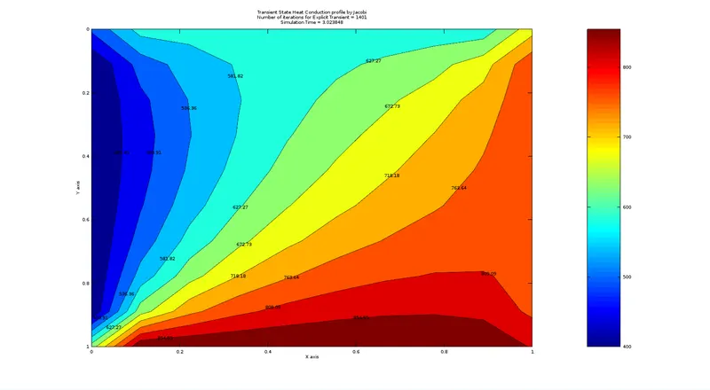
Number of Iterations for SOR = 1401

Simualtion Time = 2.98 sec

• Transient State 2-D Heat Conduction Equation Implicitly :

Implicit methods find the solution for the latter state of the equation by taking the information from the current as well as from the latter state.Therfore the unknowns appears twice in the implicit equations and the equation becomes linear coupled equation.

The Implicit Schemes are very stable and sustain stability at large time-steps.

eq(2) when discretized for the implicit scheme will be ;

`(delT)/(delt) = alpha (del^2T)/(delx^2)+ (del^2T)/(dely^2)` ------(2)

`(T_p^(n+1) - T_p^n)/dt = alpha((T_l^(n+1)-2T_p^(n+1)+T_r^(n+1))/dx^2 + (T_t^(n+1) - 2T_p^(n+1)+T_b^(n+1))/dy^2)`

From above equation we see that the terms of the spatial terms also occurs in the latter state and makes the equation coupled with (n) and (n+1) state occurs together in the equation and making it difficult to solve without Iterative solvers.

rearraning the terms we will get,

`T_p^(n+1) = 1/(1+2k1+2k2)[T_p^n +k1(T_l + T_r)^(n+1) +k2(T_t + T_b)^(n+1)]`

now we can reduce the equation in terms and can solve it for all the three Iterative Methods,

term1 = `1/(1+2k1+2k2)`

term2 = `term1*k1`

term3 = `term1*k2`

H = `(T_l + T_r)`

V = `(T_t + T_b)`

The H and V terms for jacobi and gauss-seidel will be as follows

• for jacobi: H = `(Told_(i-1,j) + Told_(i+1,j))` and V = `Told_(i,j+1) + Told_(i,j-1)`
• for gauss-seidel: H = `T_(i-1,j) + Told_(i+1,j)` and V = `Told_(i,j+1) + T_(i,j-1)`

`T_(i,j) = (term1*Tprev_(i,j)) + (term2*H) + (term3*V)`

where Tprev is the value of T at the prev time-step.

• Code for 2-D Heat Conduction for the Transient State Implicit Method :

% 2-D Heat Conduction Transient State Implicit method code

clear all
close all
clc

%Inputs
l = 1;
nx = 10;
ny = 10;
alpha = 1.4;                    %Thermal Diffusivity constant
dt = 0.001;                     %Time step size dt
nt = 1300;                      %Number of time steps
tol = 1e-4;                     %Tolerance


%creating 2-D mesh
x = linspace(0,l,nx);
y = linspace(0,l,ny);
dx = x(2) - x(1);
dy = y(2) - y(1);

T = 300*ones(nx,ny);       %Initial Guess Value for Temp

%Top and Bottom B.C
for i = 2:nx-1
  T(1,i) = 600;
  T(nx,i) = 900;
end

%Left and Right B.C
for j = 2:ny-1
  T(j,1) = 400;
  T(j,ny) = 800;
end

%Corners nodes B.C
T(1,1) = (T(1,i) + T(j,1))/2;
T(nx,1) = (T(j,1) + T(nx,i))/2; 
T(nx,ny) = (T(nx,i) + T(j,nx))/2;
T(1,ny) = (T(1,i) + T(j,nx))/2;

Told = T;                           %updating the conditions
T_prev = Told;                      %for value of T at previous Time-step

%Defining computing terms
k1 = alpha*(dt/dx^2);               %Courant number along x
k2 = alpha*(dt/dy^2);               %Courant number along y

term1 = 1/(1+2*k1+2*k2);            %Terms for the computation
term2 = term1*k1;
term3 = term1*k2;

printf('1.Jacobi\n2.Gauss Seidel\n3.SOR\n');
method = input('Choose the Iterative Method = ');

%Computing the values

if(method == 1)              %Jacobi Method
  tic;                       %to compute simulation time
  J_iter = 1;
  for t = 1:nt               %time loop
    error = 9e9;             %error term
    while(error > tol)       %convergence loop
      for i = 2:nx-1
        for j = 2:ny-1       %space loop
          H = Told(i-1,j) + Told(i+1,j);
          V = Told(i,j+1) + Told(i,j-1);
          T(i,j) = (term1*T_prev(i,j)) + term2*H + term3*V;
        end
      end
      error = max(max(abs(T - Told)));
      Told = T;
      J_iter = J_iter + 1;
    end
    T_prev = T;
  end
  time_j = toc;
  %plotting
  figure(1)
  colormap(jet)
  X = contourf(x,y,T);
  clabel(X)
  colorbar
  xlabel('X');
  ylabel('Y');
  set(gca,'YDir','reverse');
  txt1 = sprintf('Number fo Iteration of Jacobi = %d',J_iter);
  txt2 = sprintf('Simulation Time(sec) = %f',time_j);
  title({'2-D Transient Jacobi profile';txt1;txt2});
end 

if(method == 2)              %Gauss Seidel Method
  tic;                       %to compute simulation time
  GS_iter = 1;
  for t = 1:nt               %time loop
    error = 9e9;             %error term
    while(error > tol)       %convergence loop
      for i = 2:nx-1
        for j = 2:ny-1       %space loop
          H = T(i-1,j) + Told(i+1,j);
          V = Told(i,j+1) + T(i,j-1);
          T(i,j) = (term1*T_prev(i,j)) + term2*H + term3*V;
        end
      end
      error = max(max(abs(T - Told)));
      Told = T;
      GS_iter = GS_iter + 1;
    end
    T_prev = T;
  end
  time_gs = toc;
  %plotting
  figure(2)
  colormap(jet)
  X = contourf(x,y,T);
  clabel(X)
  colorbar
  xlabel('X');
  ylabel('Y');
  set(gca,'YDir','reverse');
  txt1 = sprintf('Number fo Iteration of Gauss Seidel = %d',GS_iter);
  txt2 = sprintf('Simulation Time(sec) = %f',time_gs);
  title({'2-D Transient Gauss Seidel profile';txt1;txt2});
end

if(method == 3)              %Successive Over Relaxation Method
  omega = 1.1;               %Relaxation Factor
  tic;                       %to compute simulation time
  sor_iter = 1;
  for t = 1:nt               %time loop
    error = 9e9;             %error term
    while(error > tol)       %convergence loop
      for i = 2:nx-1
        for j = 2:ny-1       %space loop
          H = T(i-1,j) + Told(i+1,j);
          V = Told(i,j+1) + T(i,j-1);
          T(i,j) = Told(i,j)*(1 - omega) + omega*((term1*T_prev(i,j)) + term2*H + term3*V);
        end
      end
      error = max(max(abs(T - Told)));
      Told = T;
      sor_iter = sor_iter + 1;
    end
    T_prev = T;
  end
  time_sor = toc;
  %plotting
  figure(3)
  colormap(jet)
  X = contourf(x,y,T);
  clabel(X)
  colorbar
  xlabel('X');
  ylabel('Y');
  set(gca,'YDir','reverse');
  txt1 = sprintf('Number fo Iteration of SOR = %d',sor_iter);
  txt2 = sprintf('Simulation Time(sec) = %f',time_sor);
  title({'2-D Transient SOR profile';txt1;txt2});
end 

• for the transient implicit schemes the error term is initialized inside the time loop.
• the time record for the simulation is recorded after the time loop
• to save the computational time the plotting of the contour can be written outside the time loop

• Result for Transient State Implicit scheme :
• Transient State Jacobi Method results

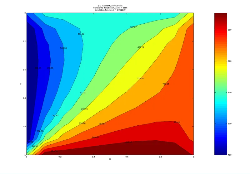
Number of Iteraion for Jacobi = 3566

Simulation Time = 5.951 sec

• Transient State Gauss-Seidel Method results

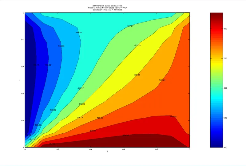
Number of Iteraion for Jacobi = 3017

Simulation Time = 4.972 sec

• Transient State SOR Method results

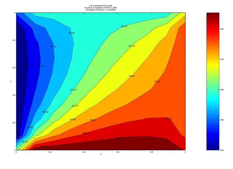
Number of Iteraion for Jacobi = 2645

Simulation Time = 5.192 sec

Conclusion :

State of Equation	Schemes	Iterative Methods	Number of Iterations	Simulation Time
Steady	------	Jacobi	208	0.29
		Gauss-Seidel	112	0.16
		SOR	60	0.10
Transient	Explicit	-----	1401	2.98
Transient	Implicit	Jacobi	3566	5.951
		Gauss-Seidel	3017	4.972
		SOR	2645	5.192

• From the results yielded for Steady State with very less number of iterations and also takes less computational time compare to the other mehods.Therefore

SOR>Gauss-Seidel>Jacobi. For steady state SOR yields solution faster and in less iterations

• For Tranisent State the simulation for Explicit and Implicit, the results are yielded quicker and in less iteration for Explicit scheme rather than Implicit.
• For Transient State Implicit SOR yield the result in less numbe of Iteration than the other two methods but the simulation time is increased as more number of number of steps has to be performed in a single time-step.
• Successive Over Relaxation method yields the result faster for both Steady and Transient Implicit State.
• For Transient Implicit scheme SOR>Gauss-Seidel>Jacobi.
• For Transient Explicit state the CFL condition has to obeyed otherwise the solution gets diverge.
• Transient Implicit Schemes can be stable for larger values of time-step size.