Week 5.2 - Literature review: ODE Stability

Introduction: A literature review of Ordinary Diffrential Equation ODE and it stability.

1. When does a ODE become unstable?

Lets assume an ODE , `f(y) = dy/(dt) = -1000y-e^-t`

this is the function of f(y,t). To answer the question we will solve this equation numerically in Python and compare the results with analytical solution.

For the given equation we will solve for analytically, numerically with explicit and implicity functions.

Explicit Function: y(k+1) = y(k) + f(y(k),t(k))dt

Implicity Function: y(k+1) = y(k) + f(y(k+1),t(k))dt

Code:

import numpy as np 
import matplotlib.pyplot as plt 
import math

def analytical(t_tot, dt):
	t = np.arange(0, t_tot, dt)
	y = np.zeros(len(t))

	for i in range(0,len(t)):
		y[i] = math.exp(-1000*t[i])*(1-math.exp(999*t[i]))/999;
	return[t,y]


def explicit(t_tot, dt):
	t = np.arange(0, t_tot, dt)
	y = np.zeros(len(t))

	for i in range(0,len(t)):
		y[i] = y[i-1] + dt*(-1000*y[i-1] - np.exp(-t[i-1]));
	return[t,y]

def implicit(t_tot, dt):
	t = np.arange(0, t_tot, dt)
	y = np.zeros(len(t))

	for i in range(0,len(t)):
		y[i] = (y[i-1] - np.exp(-t[i])*dt)/(1+1000*dt);
	return[t,y]

t_tot = 0.5
dt = 0.05

t,y_ana = analytical(t_tot,dt)
t,y_exp = explicit(t_tot,dt)
t,y_imp = implicit(t_tot,dt)

plt.plot(t,y_ana)
plt.plot(t,y_exp)
plt.plot(t,y_imp)
plt.legend(["analytical","explicit","implicit"])
plt.grid('on')
title = ('timestep:',dt)
plt.title(title)
plt.show()

Results-Conclusion:

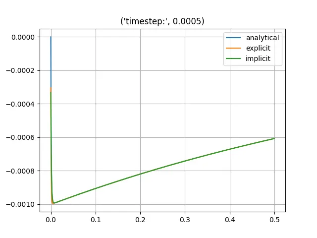
dt = 0.0005

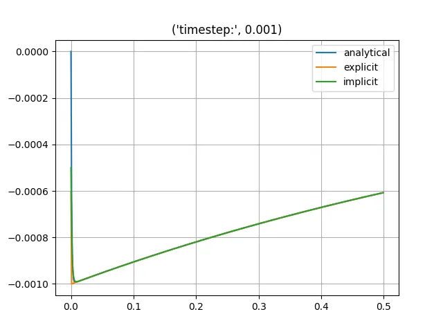
dt = 0.001

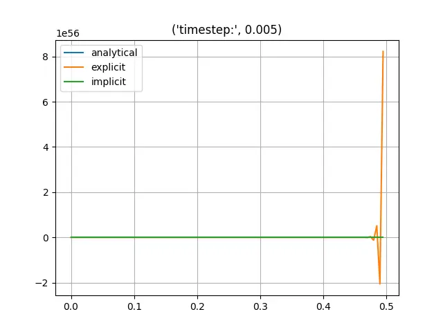
dt = 0.005

dt = 0.05

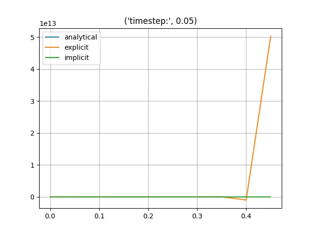
From the figures obtained from the python code we conclude that as we increase the time-step size for solving the equation the explicit function results keep distorting and provides unphysical results. While the implicit part hold good as w.k.t implicit solver are unconditionally stable. Hence for a bigger value of dt(timestep size) the ODE results become unstable.

2. How does stability affect engineering simulations?

Stability of numerical simulations strongly affects engineering simulations. It dosent matter if we are simulating fluid flows, heat transfer, combustion if the solution is unstable the results will be unphysical and of no use, as it is shown in dt = 0.05 and 0.005 graphs above.

Unstable solutions contains a lot of oscillations in the results, sudden and sharp deviation from the numerical results. If this oscillations damps and that solution reaches the appropriate tolerance values than that numerivcal results are reliable to use.

3. Can stability conditions be derived for all types of problems?

Stability conditions are very important for the explicit solving problems. Stability conditions are derived only for linear ode's, for the non-linear ode's are defined by jacobian matrix. Jacobian matrix is nothing but a matrix of first-order derivatives of all the functions w.r.t all independent variables. The eigenvalue of the jacobian matrix is computed, if eigenvalue is negative than the ode is said to be stable.