Week 6 - Multivariate Newton Rhapson Solver

Aim: To solve a coupled non-linear system of ODE's using the Multivariate Newton-Raphson Method in Python.

ODE's:

`(dy_1)/(dt) = -0.04y_1+10^4y_2y_3`

`(dy_2)/(dt) = -0.04y_1+10^4y_2y_3-3*10^7y_2^2`

`(dy_3)/(dt) = 3*10^7y_2^2`

Theory:

Multivariate Newton-Raphson Method:-
The Newton-Raphson method is root finding iterative solution, which is use to calculate the best approximation from the guess value for the function. The Newton-Raphson method is used when there is only one independet variable whereas, the Multivariate Newton-Raphson method is used when the function has two or more independent variables.

The Newton-Raphson method is calculated using the given formula:

`y_(text(new)) = y_(old) - alphaJ^(-1)F`

where α is the Relaxation Factor, J is the Jacobian Matrix, F is column matrix of functions,

`y_(text(new)) = [[y_1], [y_2], [y_3]]`

`y_(old) = [[y_(1old)], [y_(2old)], [y_(3old)]]`

The Jacobian Matrix contains all first order partial derivative of the function. It shows how output of vector valued function changes with input.

J = `[[(df_1)/(dy_1) (df_1)/(dy_2) (df_1)/(dy_3)], [(df_2)/(dy_1) (df_2)/(dy_2) (df_2)/(dy_3)] ,[(df_3)/(dy_1) (df_3)/(dy_2) (df_3)/(dy_3)]]`

F = `[[f_1],[f_2],[f_3]]`

This formula is executed untill the program reaches a better approximation for the values of y1, y2 and y3.

Program:

For our code we have some initial data:

α = 1.0

total time = 10*60 = 600s

For selection of the time-step size, if the program has to be executed with Explicit Euler method than the dt has to be small for a smooth execution of the code. But we are solving with Backward Differencing Methods/ Implicit Euler Method so the dt can be large without compromising the computation efficiency.
Therefore the choice of dt = 0.05, then the number of time-steps is given by: 600/0.05 = 12000

Also for computing the Jacobian numerically, we used the forward differencing so for calcuation for f1

`(df_1)/(dy_1) = (f1(y1+h) - f1(y1))/h`

'h' selection is very small like 1e-6

"""
Solving coupled non-linear ODE's using multivariate Newton-Raphson method

    Equations:
                dy1/dt  = -0.04*y1 + pow(10,4)*y2*y3
                dy2/dt  = -0.04*y1 + pow(10,4)*y2*y3 - 3*pow(10,7)*pow(y2,2)
                dy3/dt  = 3*pow(10,7)*pow(y2,2)

The simulation is run for 600s with dt is 0.05
"""

import matplotlib.pyplot as plt
from numpy.linalg import inv
import numpy as np
def f1(y10,y1,y2,y3,dt):

	return (y10 + dt*(-0.04*y1 + y2*y3*1e4) - y1) 
	
def f2(y20,y1,y2,y3,dt):

	return (y20 + dt*(0.04*y1 - (1e4*y2*y3) -(3e7*y2*y2)) -y2)
		 
def f3(y30,y1,y2,y3,dt):

	return (y30 + dt*(3e7*y2*y2) - y3)
		  
def jacobian(y10,y20,y30,y1,y2,y3,dt): 
	J = np.ones((3,3)) 
# Jacobian solved by numerical derivative. 
	h = 1e-6 # Step size 

	J[0,0] = (f1(y10,y1+h,y2,y3,dt)-f1(y10,y1,y2,y3,dt))/h 
	J[0,1] = (f1(y10,y1,y2+h,y3,dt) -f1(y10,y1,y2,y3,dt))/h 
	J[0,2] = (f1(y10,y1,y2,y3+h,dt) -f1(y10,y1,y2,y3,dt))/h 

	#Row 2 
	J[1,0] = (f2(y20,y1+h,y2,y3,dt) -f2(y20,y1,y2,y3,dt))/h
	J[1,1] = (f2(y20,y1,y2+h,y3,dt) -f2(y20,y1,y2,y3,dt))/h 
	J[1,2] = (f2(y20,y1,y2,y3+h,dt)-f2(y20,y1,y2,y3,dt))/h 
# Row 3 
	J[2,0] = (f3(y30,y1+h,y2,y3,dt)-f3(y30,y1,y2,y3,dt))/h 
	J[2,1] = (f3(y30,y1,y2+h,y3,dt)-f3(y30,y1,y2,y3,dt))/h 
	J[2,2] = (f3(y30,y1,y2,y3+h,dt)-f3(y30,y1,y2,y3,dt))/h 
	return J
# Defining initial guess value 
y10 = 1
y20 = 0 
y30 = 0 
# Initial error 
error = 9e9 
#Column Vector 
Y_old = np.ones((3,1)) 
Y_old[0] = y10 
Y_old[1] = y20 
Y_old[2] = y30 
# Column Vectors for F 
F = np.copy(Y_old) 
#Parameters for newton rapson method 
alpha = 1 
tol = 1e-6 
t = 600 
dt = 0.05
n = int(t/dt) 
y1 = [] 
y2 = []
y3 = []
iteration = []

iter = 1
for i in range(0,n):
	while error>tol: 
		J = jacobian(y10,y20,y30,Y_old[0],Y_old[1],Y_old[2],dt) 
# Computing the F vector
		F[0] = f1(y10,Y_old[0],Y_old[1],Y_old[2],dt) 
		F[1] = f2(y20,Y_old[0],Y_old[1],Y_old[2],dt) 
		F[2] = f3(y30,Y_old[0],Y_old[1],Y_old[2],dt) 
# Computing the new values
		Y_new = Y_old - alpha*np.matmul(inv(J), F)
		error = max(abs(Y_new-Y_old)) 
		print(error) #Updating the old values 
		Y_old = Y_new #log message 
# Storing the values for plotting 
		y1.append(Y_new[0]) 
		y2.append(Y_new[1]) 
		y3.append(Y_new[2]) 
		iter = iter + 1
		iteration.append(iter)
		Y_old = Y_new
		y10 = Y_new[0]
		y20 = Y_new[1]
		y30 = Y_new[2]

plt.plot(iteration,y1, color = 'green')
plt.plot(iteration,y2, color = 'red')
plt.plot(iteration,y3, color = 'black')
plt.xlabel('Number of Iterations')
plt.ylabel('Variables')
plt.legend(['y1','y2','y3'])
plt.title('Solution for ODE System')
plt.grid()
plt.show()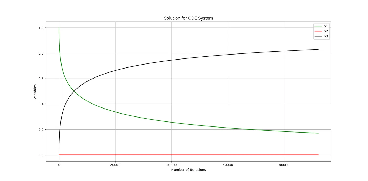

Conclusion: Hence, the Newton-Raphson method solver is programmed in Python and the set of coupled non-linear three ODE's and the graph for y1, y2 and y3 against iteration for convergence.