Week 5 - Rayleigh Taylor Instability
Aim : To simulate and analyze Rayleigh Taylor Instability of air and water material and state the effects of Atwood number and changes in grid on the instabilities.
Introduction :
MULTIPHASE : Multiphase flow is a simultaneous (parallel) flow of materials with different states or phase (liquid-gas).
It is a flow of materials with different chemical properties but in the same state or phase (liquid-liquid). there are 3 types of flows in MULTIPHASE.
multiphase flow analysis simulation is used to accurately predict the simultaneous interacttion of more than one combination of phases that can be solid , liquid,gases. Multiphase flows are often an important method of heat and material transport . two phase flow determines the process in steam generators,condesators and cooling towers of steam power operation.
1. Liquid-gas flow : water-water vapour in heat pipe
2. liquid-solid flow : turbulent binghamian slurries
3. gas-solid flow : pnuematic transport
types of phase in multiphase are :
1. separated phase : it is defined as one or more immiscible fluids in a continious phase separated by an interface.
2. mixed phase : is defined as a phase in which one or more fluids mixed together .it contains both separated and dispersed phase.
3. dispersed phase : it is defined as the phase in which the finite number of phases are seprated in the continous phase.
As multiphase flows are very important in industrial workings, automobile and many more industries to solve the multiphase problems numerically there are different models are used to solve the multiphase problems and analyze them more accuratley. to approach such problems the models used in CFD are ;
1. The VOF model :
The VOF model is a surface-tracking technique applied to a fixed Eulerian mesh. It is designed for two or more immiscible fluids where the position of the interface between the fluids is of interest. In the VOF model, a single set of momentum equations is shared by the fluids, and the volume fraction of each of the fluids in each computational cell is tracked throughout the domain. Applications of the VOF model include stratified flows , free-surface flows, filling, sloshing , the motion of large bubbles in a liquid, the motion of liquid after a dam break, the prediction of jet breakup (surface tension), and the steady or transient tracking of any liquid-gas interface.
2. The Mixture Model :
The mixture model is designed for two or more phases (fluid or particulate). As in the Eulerian model, the phases are treated as interpenetrating continua. The mixture model solves for the mixture momentum equation and prescribes relative velocities to describe the dispersed phases. Applications of the mixture model include particle-laden flows with low loading, bubbly flows, sedimentation , and cyclone separators. The mixture model can also be used without relative velocities for the dispersed phases to model homogeneous multiphase flow.
3. The Eulerian Model:
The Eulerian model is the most complex of the multiphase models in ANSYS FLUENT. It solves a set of momentum and continuity equations for each phase. Coupling is achieved through the pressure and interphase exchange coefficients. The manner in which this coupling is handled depends upon the type of phases involved; granular (fluid-solid) flows are handled differently than nongranular (fluid-fluid) flows. For granular flows , the properties are obtained from application of kinetic theory. Momentum exchange between the phases is also dependent upon the type of mixture being modeled. ANSYS FLUENT's user-defined functions allow you to customize the calculation of the momentum exchange.Applications of the Eulerian multiphase model include bubble columns , risers , particle suspension, and fluidized beds .
Rayleigh Taylor Instabilty:
The Rayleigh Taylor Instability or RT instabilty is an instability of an interface between two fluids of different densities which occurs when the lighter fluid is pushing the heavier fluid . example like behavior of waterrr suspended above oil in the gravity of earth , mushroom clouds like those form from volcanic eruption and many more.Rayleigh Taylor instability can be molded by two completely plane parallel layerrs of immiscible fluid, the denser fluid on the top of the less dense fluid and both are subjected to earths gavity. the equillibrium here is unstable to any disturbances of the interface, if the parcel of the heavier fluid is displaced downward with an equal volume of lighter fluid displaced upwards. this situation is equivalent to the situation when the fluids are accelerated, with the less dense fluid accelearating into denser as
the RT instability develops , the initial disturbance progress from a linear growth phase into a non-linear growth phase,eventually developing "plumes" follwoing upwards and "spikes" falling downwards.in general, the density disparity between the fluids determines the structure of the non linear RT instability flows.
the changes in the RTI follows four main stages. the peturbation amplitudes are small when compared to thier wavelenghts, the equation of motion can be linearized, resulting in exponential instability growth. In the early portion of this stage, a sinusoidal initial perturbation retains its sinusoidal shape. However, after the end of this first stage, when non-linear effects begin to appear, one observes the beginnings of the formation of the ubiquitous mushroom-shaped spikes (fluid structures of heavy fluid growing into light fluid) and bubbles (fluid structures of light fluid growing into heavy fluid). The growth of the mushroom structures continues in the second stage and can be modeled using buoyancy drag models, resulting in a growth rate that is approximately constant in time. At this point, nonlinear terms in the equations of motion can no longer be ignored. The spikes and bubbles then begin to interact with one another in the third stage. Bubble merging takes place, where the nonlinear interaction of mode coupling acts to combine smaller spikes and bubbles to produce larger ones. Also, bubble competition takes places, where spikes and bubbles of smaller wavelength that have become saturated are enveloped by larger ones that have not yet saturated. This eventually develops into a region of turbulent mixing, which is the fourth and final stage in the evolution. It is generally assumed that the mixing region that finally develops is self-similar and turbulent, provided that the Reynolds number is sufficiently large.
ATWOOD NUMBER :
The Atwood number (A) is a dimensionless number in fluid dynamics used in the study of hydrodynamic instablities used in density stratified flows. it is a dimensionless density ratio defined as differnce in density of heavier fluid and lighter fluid to the sum of the densities of the heavier and lighter fluid.
A = ρ1 - ρ2 / ρ1 +ρ2
where , ρ1 = density of heavier fluid
ρ2 = density of lighter fluid
for A close to 0 ,RT instability flows take the form of symetric "fingers"of fluid and for A close to 1, the much lighter fluid below the havier fluid takes the form of larger bubbles like plumes.
Requirement : Case 1 :perform grid test with base mesh of 0.5mm and one reine mesh of 0.3mm and compare results and show the animation.
Case 2. run other mesh with user-defined material with the density =400kg/m^3 and
viscosity = 0.001kg/m-s
Procedure for the simulation:
1. geometry setup in spaceclaim : we will create the geometry in the ansys fluent spaceclaim
to create the 2d geometry for the simulation, we will create two squares of 20*20 mm of lenght in the same plane
then we will use the Pull option to convert the sktech into the surface and then we will create another square on top of the other.
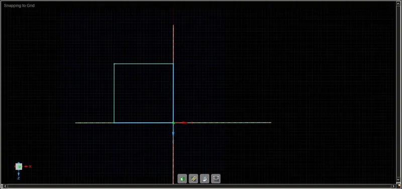
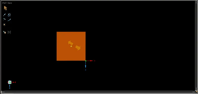
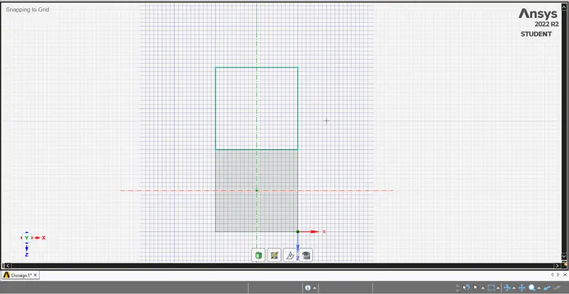
after the squares are created we have to make sure that the topology of the geometry is shared otherwise we will again encounter the non-conformal mesh.
go to Workbench > share > select both squares > click ok.
after the sharing is done we can confirm it by seeing in the full geometry right click on it and in the left side box we can see that the topology is shared and other way to confirm the sharing is looking under the name Design we can see the icons with pink colour line indiccating the sharing.
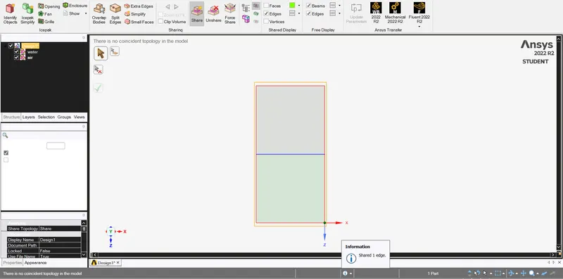 with this we are done with creating the geometry.
2. Mesh Setup : we will run mesh with a baseline mesh lenght of 0.5mm and one more with refine mesh of 0.3mm. for the mesh lenght reducing to 0.2 or 0.1 mm we will face the problem of floating exception point error and for the structure that is straight doing very refine mesh will create problem.
to generate the mesh lenght go to mesh > element size = 0.5mm base mesh > generate mesh.
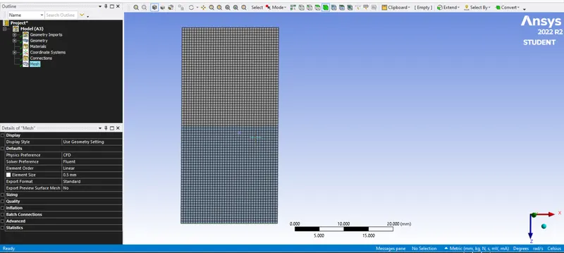 0.5mm mesh lenght
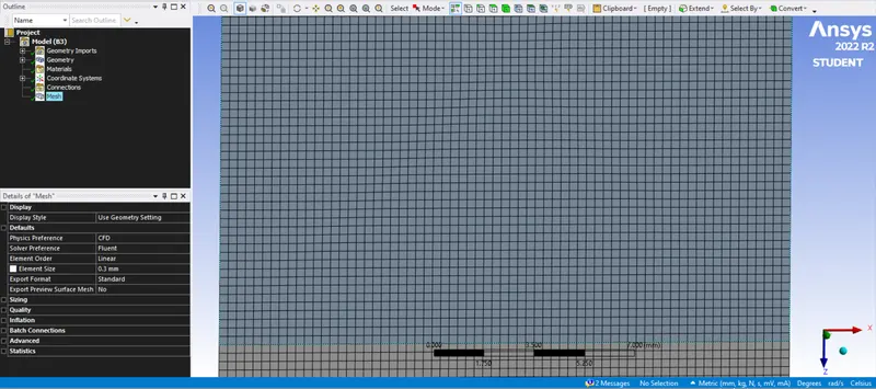 0.3mm mesh lenght
here the mesh setup is done now we will setup the physics and run the simulation.
3. Fluent Setup :
set up the physics with the requirements:
pressure based , absolute velocity
transient state
Explain why a steady-state approach might not be suitable for these types of simulation
The state in which the behavior or the parameters (density,viscosity,pressure) of the fluid changes with time is called a transient or unsteady state and the state in which the fluid parameters do not change with time is called steady state. For the rayleigh taylor instability is a time dependent behaviour of fluid. the instability of the fluids changes with time therefore the transient state is a suitable choice to simulate this challenge.The instabilities changes exponentially with respect to time .On the other hand steady state simulation is used when the simulation is focused on the end result, though the steady state will capture those instabilites but the result will not be time accurate.
turn on gravity that will act in negative y direction Y = -9.81
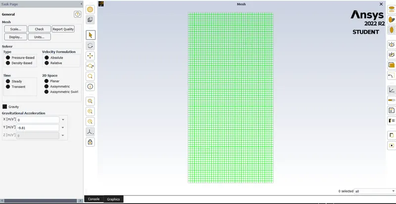
we will use the Laminar model for this simulation.
to set the Multiphase model
multiphase > volume of fluid method > implicit > ok.
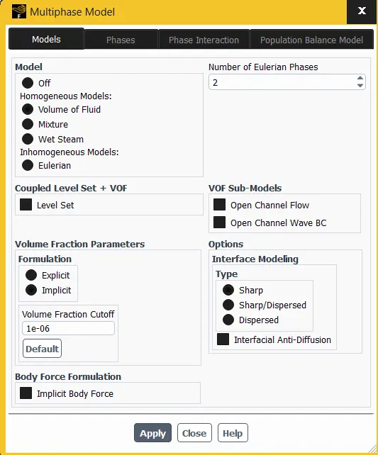
we will use 2 material for the heavier fluid = water and lighter fluid = air with the desnities of water and air is 1.225 kg/m^3 and 998.2 kg/m^3 respectively.
we will also set the phases as primary and secondary
go to multiphase > phases > set air as primary phase and water as secondary phase > ok.
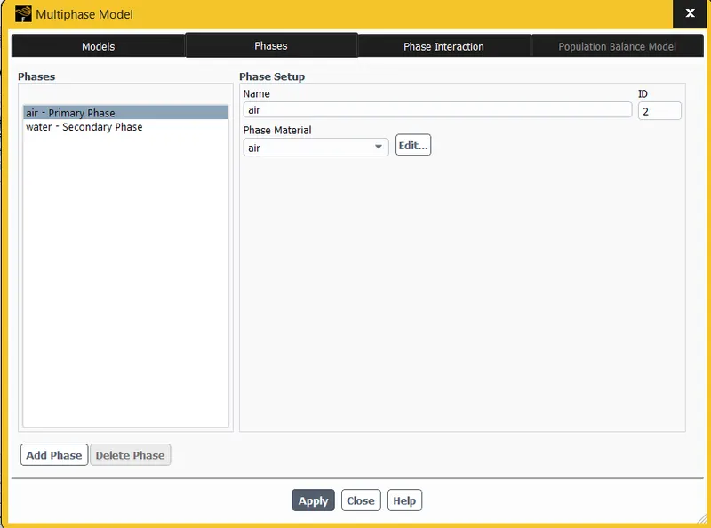
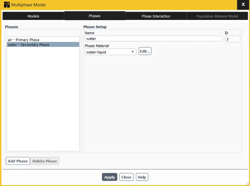
Now we will set the water phase in the top wall to set this we will do the initialization and then we will use the Patch option so that the water will remain in the upper side.
Patch > phase : water > volume fraction > set the volume = 1 and select the top wall > and set = 0 for the bottom wall > ok.
also create contours for the phase water and also create the animation solution for the phase water contour.
Run the simulation and plot the animation results.
Result : Case 1 (a) base mesh = 0.5mm
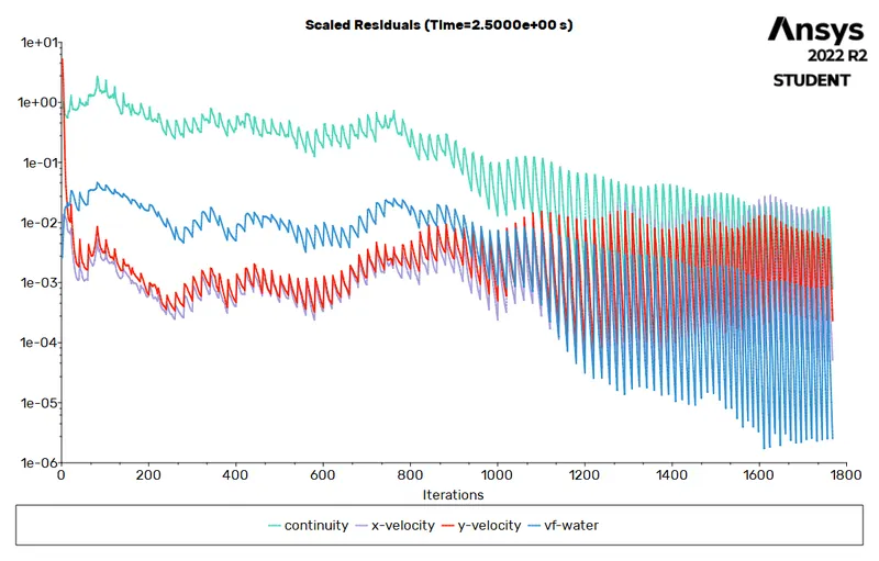
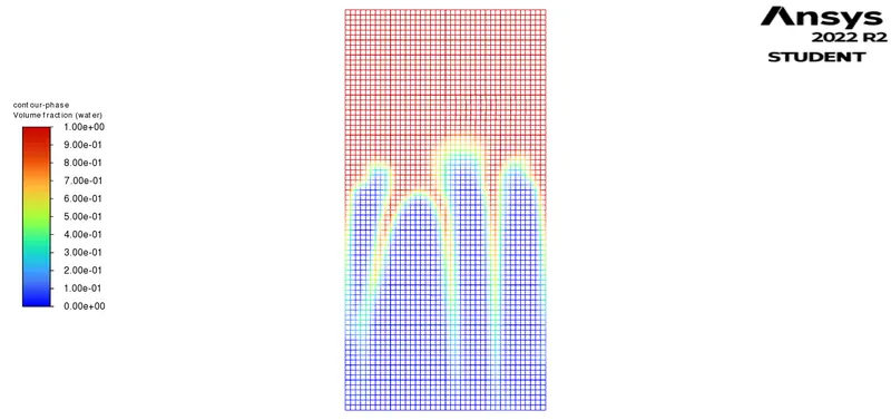
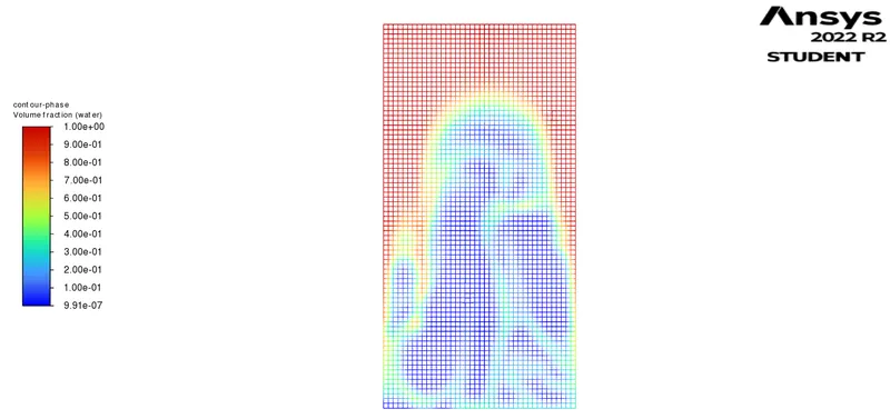
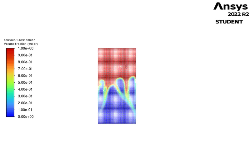
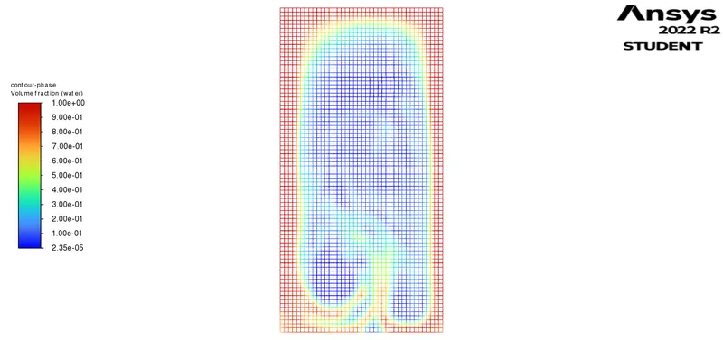 these images are from the animation the red phase represent water at the top in the beginning and air in the bottom as both phases are subjected to earth gravity the interface becomes unstable and we see very small instabilities at the interface then those are incresed as exponentially and becomes on linear as the air accelerates throuht the heavier fluid it makes plumes like or droplets like forms and the water takes spike like formation.
link for the animation file is attached below for the base mesh.
https://drive.google.com/file/d/168cxQB6SE2-iNw-T7FtOOrRHEGgeaTIl/view?usp=share_link
Case 1 (b) Refined mesh = 0.3mm
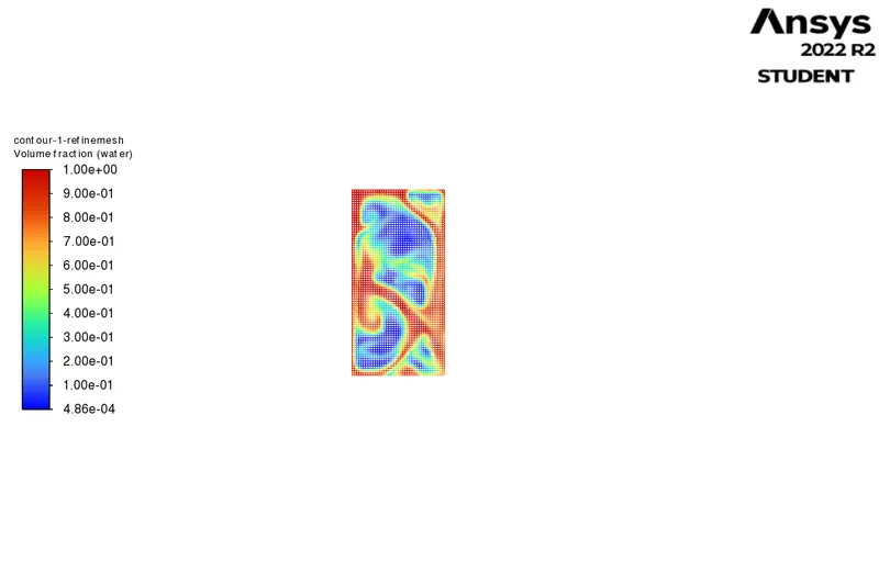
Atwood Number for the a, b for Case 1 is 0.997
that is closer to 1 thats why we are able to see the plumes like form created by the lighter fluid under the heavier fluid.
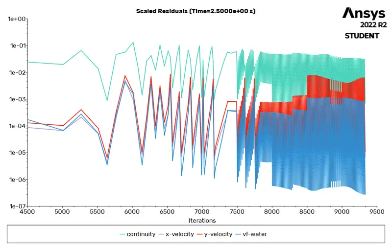
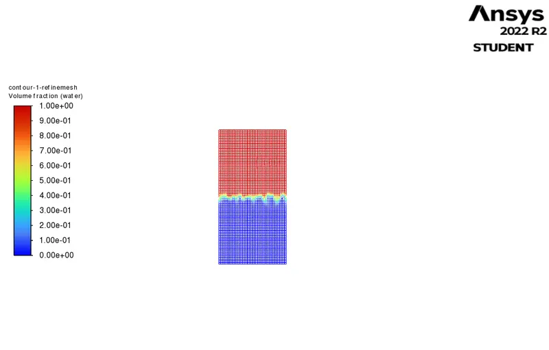
the link for the refined mesh is pasted here:
https://drive.google.com/file/d/1MY0PKY_ha7KHZAaUH4KZigdslUYQ4JH3/view?usp=share_link
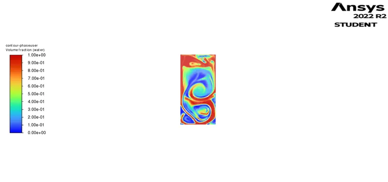
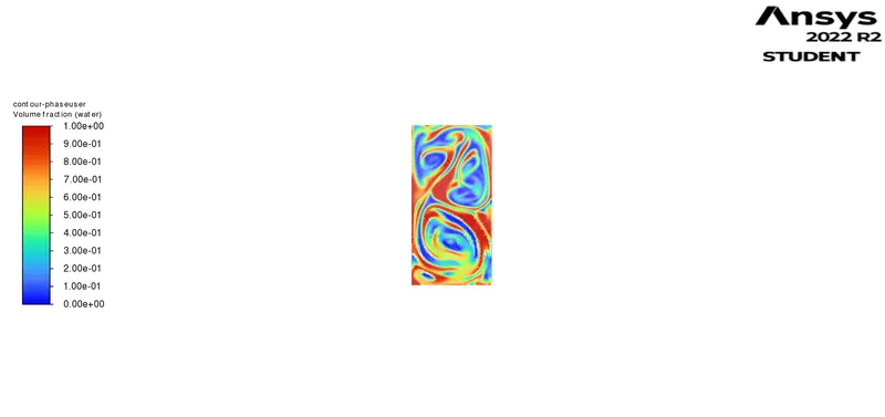
2. Case 2 : user defined material with the density = 400 kg/m^3 and viscosity = 0.001kg/m-s
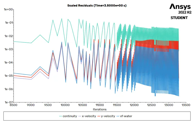
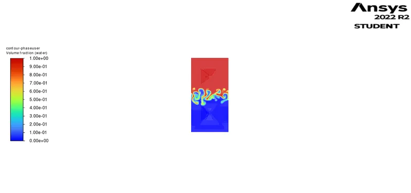
Atwood Number A = 0.427
the link for the animation for the user defined material case is mentioned down below:
https://drive.google.com/file/d/1etOs-3jkyj8_icktxfT6Fr1x3LEGe1YB/view?usp=share_link
Conclusion : In the first case study with the baseline mesh Case 1 (a) the result prodecued is from coarse mesh though it gave the conformation of the case setup is correct and the fluid behaviour can be seen unstable. But the result lack in resolution as the mesh was coarser it didnt capture the interface properly and most of the instabilities advanced in time step. The pertubations at the interface was seen a little early or premature as we know the instabilities are very small in the initial and grows exponentially but in our case we can see the disturbance assymetrical and early. due to coarser mesh the cells did not capture the interface properly and that causes inappropriate capture of instabilites at the interface.
where with case of finer mesh the result obtained were very fine. this is because the more number of cells capture the volume of fluid properly with each time step and the instabilities were captured propely right from the interface. the instabilities grows exponentially and the simulated result look realistic as compared to results obtained from the case 1 (a).
For Case 2, the case setup is same with the same refiend mesh but with different densities or Atwood Number. the larger density ratio results in stronger force to develop the interface instability.
For the case 2 with smaller Atwood Number, the density level between two sides of the interface is small. The initial desnity stratifcation plays an important role and the expansion has littile influence.with increase in Atwood Number in Case 1 the expansion compression effect becomes more significant as the difference in the density is very much high that cases the instabiltiy on the inerface increses more rapidly and signifiantly. Also larger Atwood Number results in larger amplitude of pertubation.
Also the mesh size also varies the result as the wee see in the coarser mesh case we see that the mesh do not captures the interface properly and that results in thick interface which inturn impacts difffernce in result, as some of the instabilities are not captured properly. so implentation of finer mesh with smaller time steps gave promising results.