Week 1- Mixing Tee
Aim: to perform a steady state simulation to compare the mixing effectiveness in a short and long version of MIXING-Tee when hot inlet temperature in 36°C and cold inlet temperature is 19°C for different momentum ratio.
Requirements and Formulas :
1.Short and Long Mixing Tee models
2.Formula for finding Tmixture:
Tmixture = Mhot ×Thot +Mcold×Tcold ÷ Mhot + Mcold
3. Momentum Ratio = velocity at cold inlet ÷ velocity at hot inlet
momentum values of 2,4 for both long and short mixing tee
Introduction : Ansys Fluent :
Ansys Fluent is a multipurpose Computational Fluid Dynamics (CFD). It is used to model fluid flows,heat mass transfer and chemical reations.Fluent provides cfd steps from Pre to Post Processing workflow in a single window.Fluent is known for its advanced physics modeling capabilities, which include turbulence modeling,combustion and more.Fluent also offers highly scalable, high performance computing to help solve complex, large-model CFD simulations quickly and cost-effectively. Ansys have large use over every field of civil,marine,sports,medical and more.
Mixing Tee:
Mixing Tees utilizes a specifically engineered internal geometry to efficiently mix two fluid streams into one combined stream.
The geometry of mixing tee constitutes of T-shaped mixer in which the two inlets join perpendicularly the mixing channel.
Applications of mixing tee includes low viscosity mixing such as wastewater treatment and blending of some oils (injection of additives) and petrochemical products.these mixing tee are specifically designed for high pressure applications.
Calculations : 1. calculation for velocity at cold inlet for short tee for momentum ratio of 2,4.
a. for momentum ratio of 2
momentum ratio = velocity at cold inlet ÷ velocity at hot inlet
2 = velocity at cold inlet ÷ 3
velocity at cold inlet = 6m/s
b. for momentum ratio of 4
momentum ratio = velocity at cold inlet ÷ velocity at hot inlet
4 = velocity at cold inlet ÷ 3
velocity at cold inlet = 12m/s
2. calculation for velocity at cold inlet for long tee for momentum ratio of 2,4
a. for momentum ratio of 2
momentum ratio = velocity at cold inlet ÷ velocity at hot inlet
2 = velocity at cold inlet ÷ 3
velocity at cold inlet = 6m/s
b. for momentum ratio of 4
momentum ratio = velocity at cold inlet ÷ velocity at hot inlet
4 = velocity at cold inlet ÷ 3
velocity at cold inlet = 12m/s
3. calculating the Tmixture for both momentum ratio of 2,4
Tmixture = Mhot ×Thot +Mcold×Tcold ÷ Mhot + Mcold
here, M = mass flow rate = density of air*velocity of air*area of cross section of pipe
density of air = 1.225kg/m^3
area of cross section = π/4 *d^2
a. Tmix value for momentum ratio of 2
Mcold = 0.001786
Mhot = 0.003297
therefore, Tmix = 0.003297*36 +0.001786*19 ÷ 0.003297+0.001786
Tmix = 30.02°C (Analytical value)
b.Tmix value for momentum ratio of 4
Mhot = 0.003297
Mcold = 0.003573
Tmix = 0.003297*36 +0.003573*19 ÷ 0.003297+0.003573
therefore, Tmix = 27.15°C (Analytical value)
Procedure : 1. open the ansys workbench. in ansys workbench find the ansys fluent mode in the left side of the interface and drag it to the window.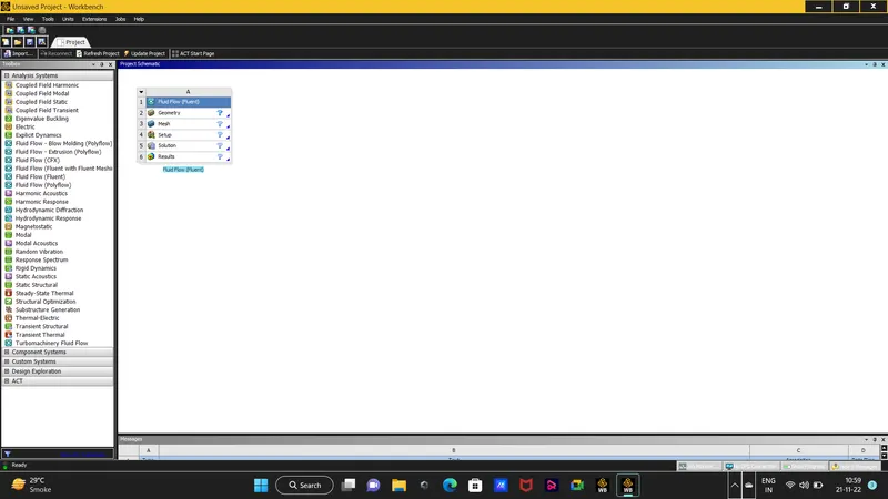 after you have drag the FLUID FLOW (FLUENT) in the window you will see a number of steps. these steps are the worflow of CFD right from pre-processing to post-processing.ansys provides a good systeematic workflow from setting up the geometry, then meshing,setting up the solution and then pre-processing the result.
2. in the geometry section for our model we will import the short mixing tee first and do all the simulation for that and then we will proceed for the long mixing tee.
3.we will import our geometry in the fluent and we can edit our geometry in the Spaceclaim editor.in spaceclaim we can edit our geometry ,we can measure the faces extract volume and more.
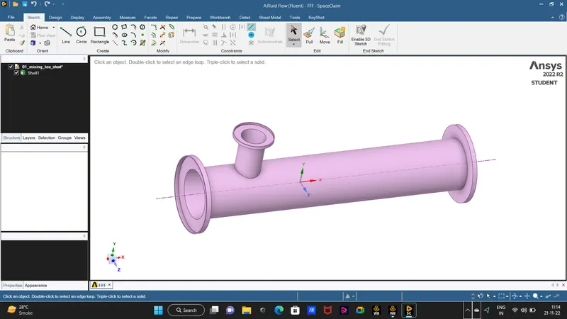 this is the spaceclaim interface.
4.in the above image we can see that our geometry is 3d as we dont want the outside geometry for our simulation, for our simulation the main flow domain is the fluid volume. fluid volume is defined as the space or volume occupied by the volume of the fluid. so we will try to delete the outside geometry but instead we can try to extract the volume as the deleting can consume more time. to extract the volume go to PREPARE > Extract Volume > select face option > select the inlet x, inlet y, outlet face > click on the green right tick to confirm the selection.
as the extraction process is done we can see in our geometry tree that there are two volumes those are Shell 1 and volume. as we dont want the shell region to com in our latter steps we will compress that geometry by right clicking the shell 1 are selecting the supress option.
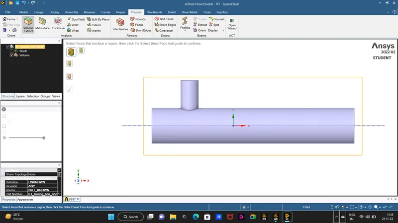 this is how the fluid volume looks.we repeat the same process for the long mixing tee.
5.as we have edited the geometry we will close the spaceclaim and we will start our mesh process by double clicking the the mesh the in the fluent box.in the mesh gui first step we will perform is to name our faces that will also help for the latter step while applying the boundary conditions. to name the faces in the mesh gui we will first select the faces option by selecting cntrl+ F. we will select the hot inlet that is in the x direction and by clicking the 'N' we will see a pop up box in which we will give the name for our inlet as inlet-x. the same process will get repeat for the inlet-y,oulet and for the walls.
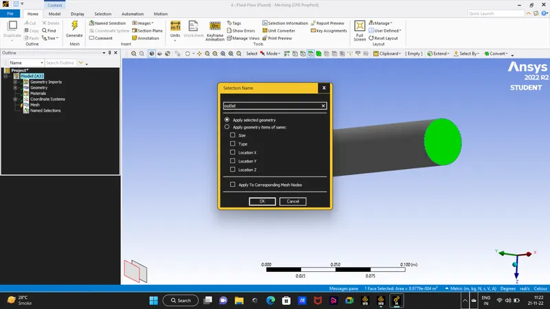
6. after naming the boundaries we can proceed the mesh. go to the mesh option in the tree section and by right clicking on the mesh then click on the generrate mesh. the mesh our geometry will get updated.
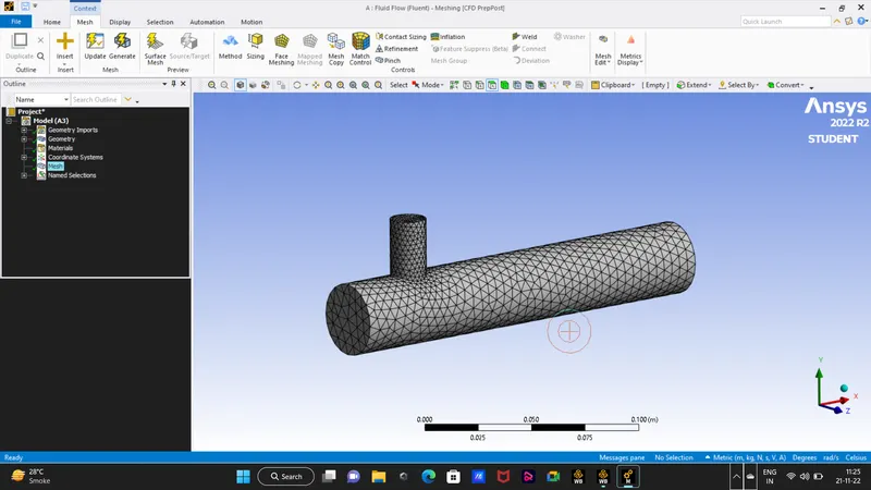 this mesh generated is a coarse mesh as it is updated on our geometry.we will now check the element quality of the mesh generated by selecting the quality option in the left window and select mesh metric >element quality>a chart of mesh metrics will appear on which the x directon = element metrics and on y axis = number of elements.
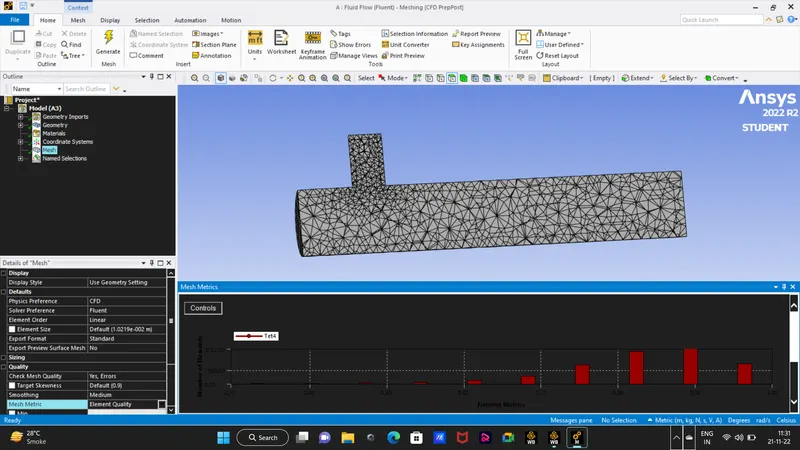 by checking our chart we can see that the quality of our mesh is 0.5 i.e 50% so now we can update our mesh and we can proceed for our setup stage.
7. close the mesh window and double click the setup process . in setup process we do work of setting up the physics like mentioning the what type of state the fluid is,to select whether model behaviour is viscous or inviscid setting up the physical model, selecting the what type of material is the fluid is , mentioning the boundary conditions , intialization , monitouring the result is the steps those are include in the setup stage.
8. in the setup stage we will setup the physics first by selecting the solver as Steady > Pressure Based > Absolute, for our mixing tee case we also want to find out the outlet temperature so we will select the energy model.
for this challenge we will expermient for two turbulence model (a) k-epsilon and (b) k-omega model these are RANS (Reynolds Average Navier Stokes) model for the short tee of momentum ratio of 2 we will select the k-epsilon model
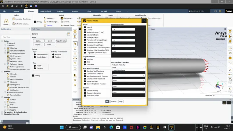 with realizable and standard wall function.
9. as we done with setting up the physics we will now give the material of the fluid as air in the Material section and then we will go by mentioning the boundary conditions. the boundary conditions are to define the problem that results in the unique solution, you must specify the infomaton on the dependent flow variables at domain boundaries.in our case the domain boundaries are inlet-x,inlet-y,outlet and walls.
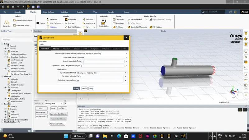 for our case the boundary conditions on our inlet x and y are the velocity inlet. for momentum ratio of 2 we will input the velocity of cold inlet as 6m/s an for hot inlet it will be 3m/s and also we will mention the temperature.
for our outlet the boundary condition will be pressure outlet.
10. as our the physics is set up and now we want to check the temperature and the standard deviation on our outlet of the mixing tee.to do that
go to Solving > Definations > New > Surface Report > Area Weighted average > temperature > outlet >create report and create file > ok
same process gets repeat for the standard deviation report.
11.now we will mention the initial condition for each solution field by selectiong the hybrid process and we can see in the console we have 10 iterations.
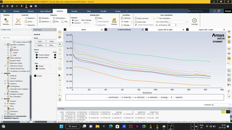
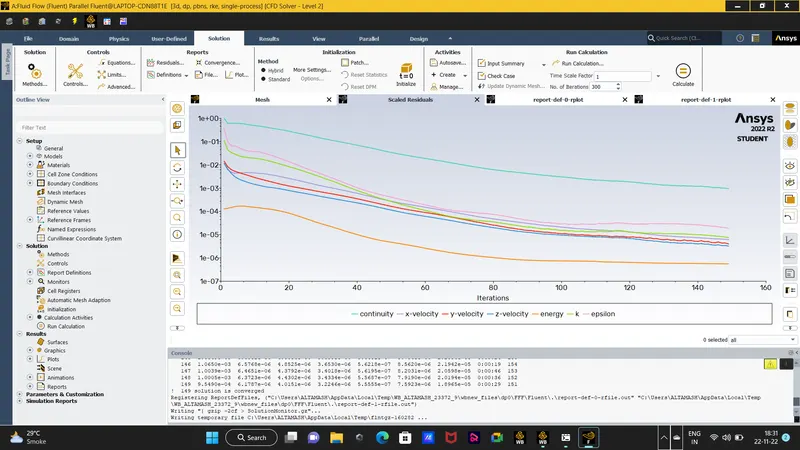
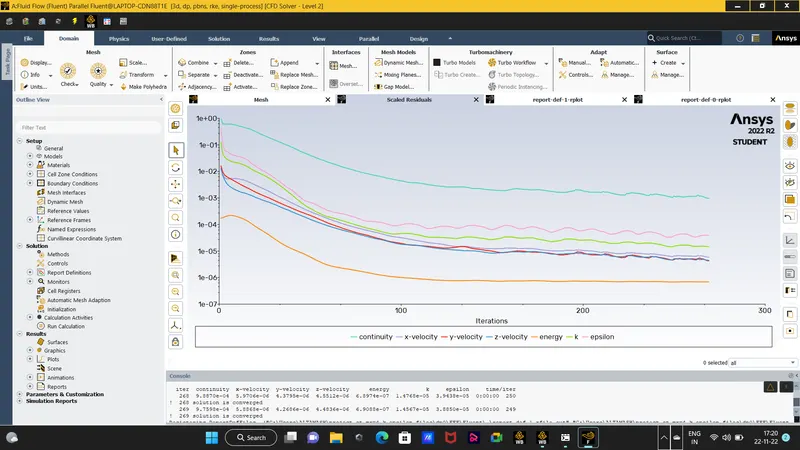
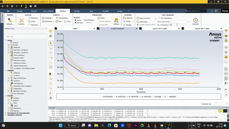
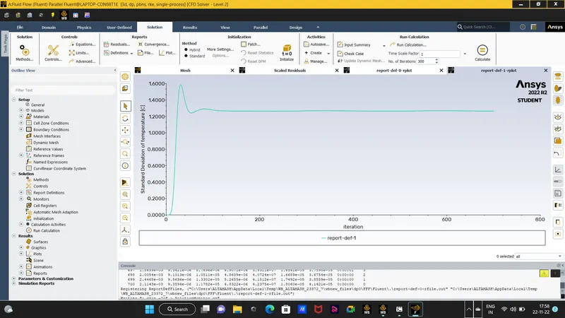
12.now we are ready to run the solution , enter the number of iteration you want in my case we runned 300 iteraions and hit calculate. as solving is done we can see graphs of sacled residual and the report that we define in the definations.
13. now we will post process our results and draw the necessary graphs and results as required for our report in the post process setup.
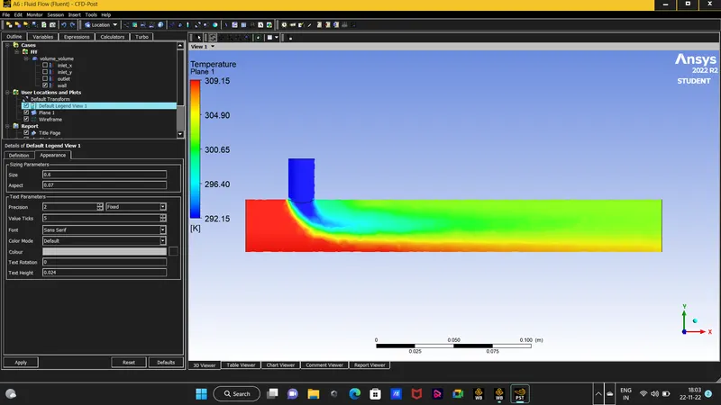
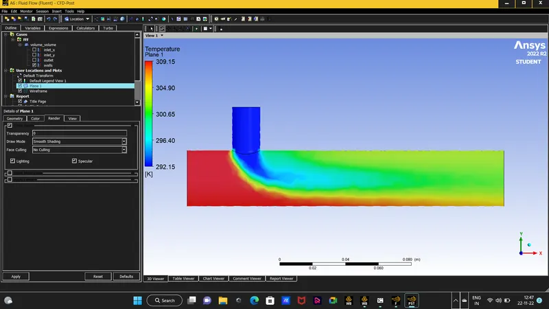 results like this are obtained in the post process
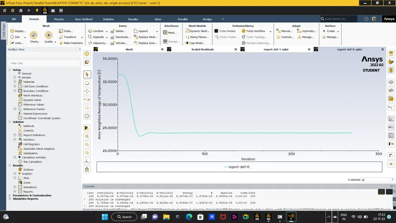
14. We run two different turbulence models for the short tee for momentum ratio of 2 .
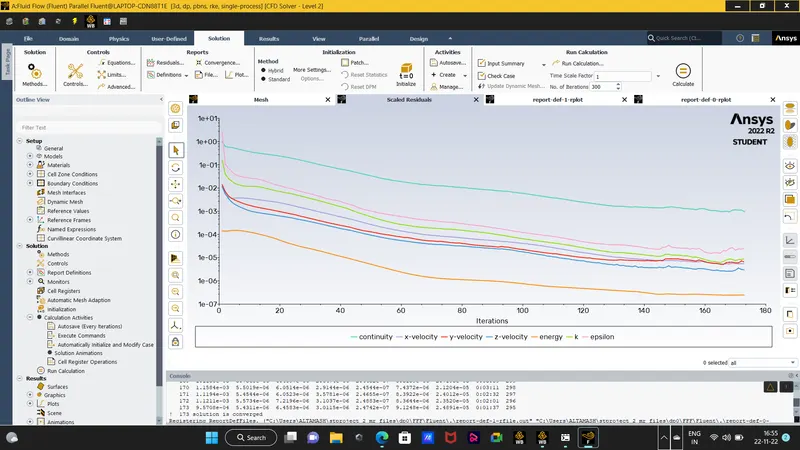
(a) short tee momentum ratio = 2 , k-epsilon model the solution converged at 165 iteratons.
temperature computed = 30.1°C
std deviation =1.17
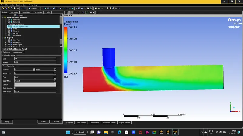
temperature plane for k epsilon model.
(b) short tee momentum ratio = 2 , k-omega model
temperature computed = 30.3°C
std deviation = 1.20
we ahd to run the solution for the 500 iterations and by checking the sacled residual we concluded the solution got converged.
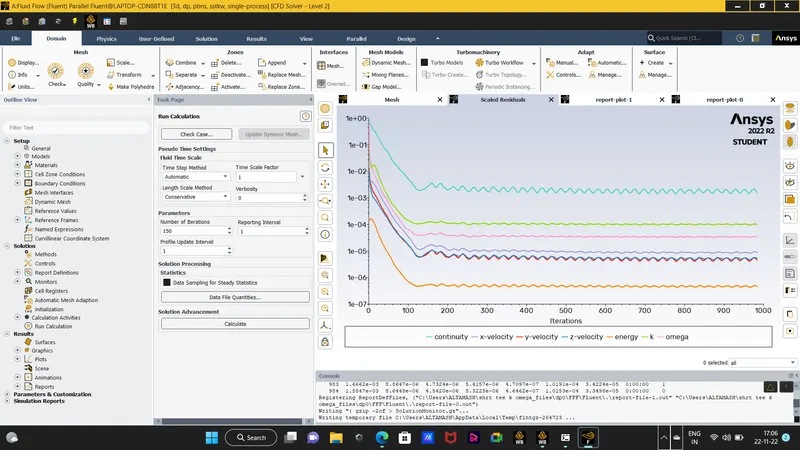
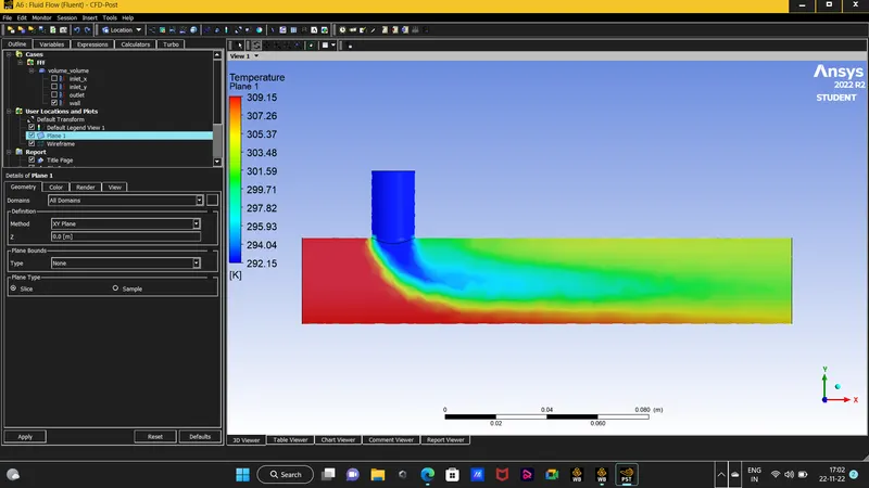
by looking at the results yield from the k- epsilon and omega model we can see that there is not much differences in the temperature and in the standard deviation.but the number of iterations computed for the solution to get converged is very high for k-omega model. the convergence tolerance for the residual for the k-epsilon is e-4 but for the k-omega the tolerance is e-3 and also the k-omega model is well suited for simulating flow in the viscous sub layer while the k-epsilon model is ideal for predicting flow behaviour in regions away from the wall which is well suited for our mixing tee challenge. So by checking all the pros and cons of the two models we will proceed with the K-epsilon model for the rest of our cases.
15. proceed to simulate all the cases with the k-epsilon model.
Tabular Coloumn :
CASES CELL NUMBERS Average Outlet Temperature Number of Iterations for Convergence
Short tee MR=2 12692 30.3°C 165
Long tee MR=4 15635 27.4°C 149
Short tee MR=4 12701 27.5°C 269
Results :
Grid Independence Study : grid independece study is conducted to learn whether the simulation is independent of the mesh or not. i used the short mixing tee mr=4 to study the normal element size was
(a) 1.0e-2m : temperature = 27.5°C and the std deviation = 0.985 with cell number of 12701 and the solution got convergedd at 268 iteration
(b) when the elements size changed to 5e-3 : the number of cells is 14138 and the solution got converged at 250 iteration but the temperature yield = 27.5°C and the std deviation = 0.809 as we see the temperature and the std deviation results dosent have much change.
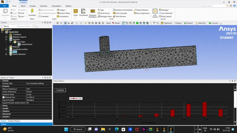 mesh for 5e-3
(c) as we further changed the mesh size to 2e-3 i.e 0.002 the number of cells increased to 106587 cells and the solution got converged at 209 iteration the temperature = 27.5°C and the std deviation = 1.09
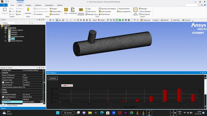 mesh size of 2e-3 the mesh adapt the geometry very well.
when we compare all three mesh size results and compare the temperature and standard deviation we see that there isnt much changes in the temperature and std deviation values and we know that as the mesh size gets finer the result accuracy increases but in our case we can go for the coarse mesh as it dosent take much computation time and still gives a much accurate result. but the post process result of the temperaturefof the 2e-3 is much more finer than the coarse mesh of 1.0e-2.
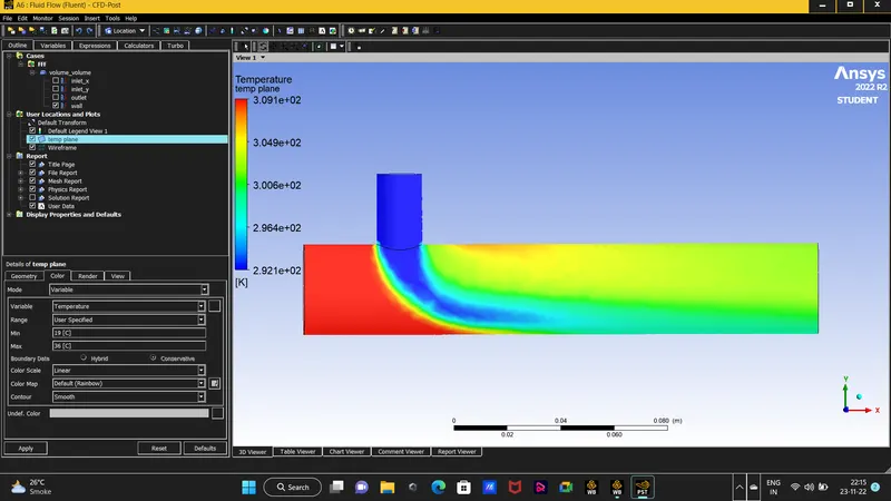 temperature post process result for 2e-3.
2.velocity and temperature countour and cut planes result:
for short tee mr = 2
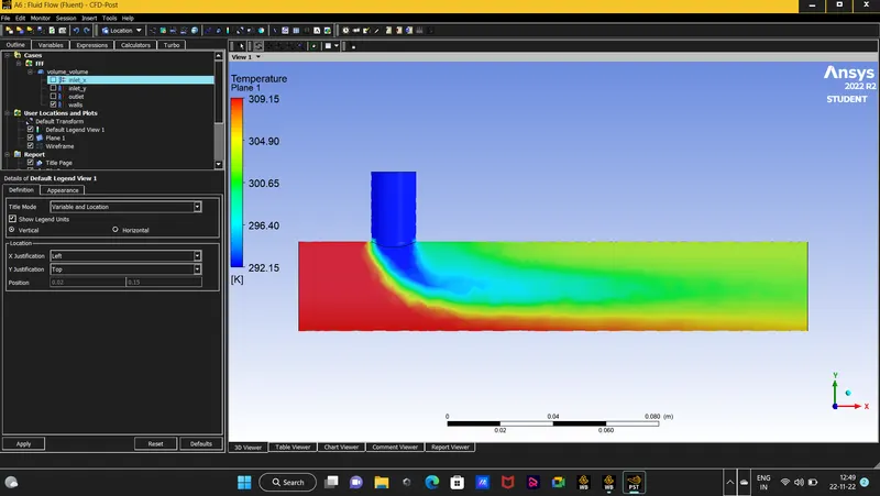
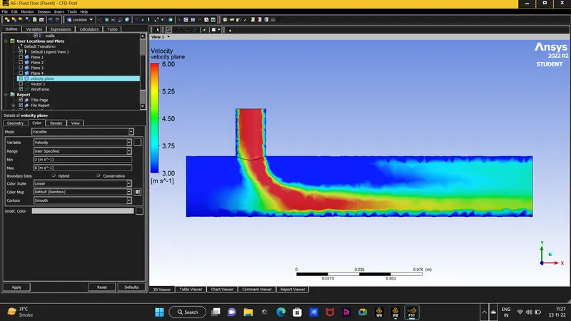
xy pots for short tee mr = 2
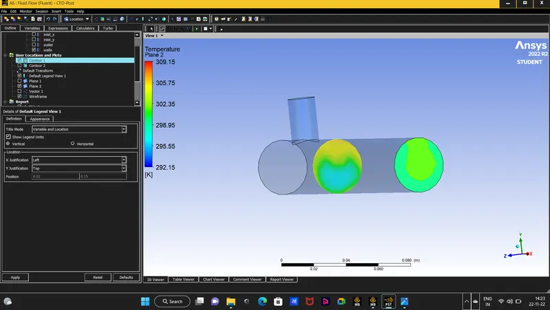
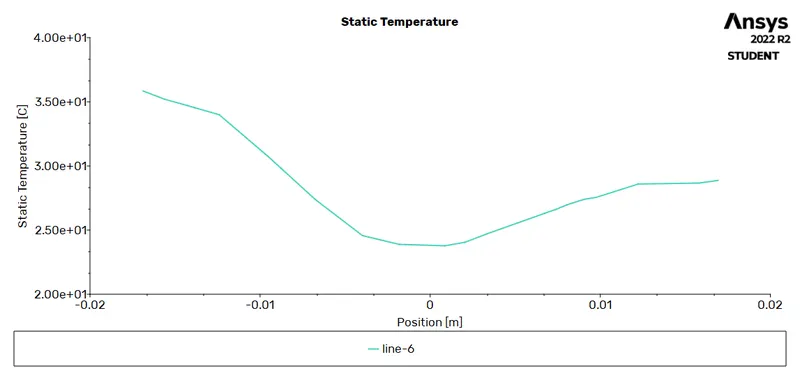 temperature across the pipe
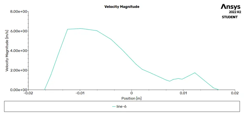 velocity across the pipe.
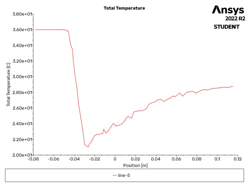 temperature along the pipe
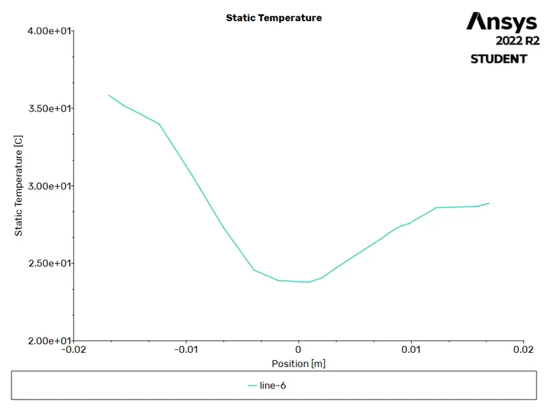 velocity along the pipe
for long tee mr = 4 results
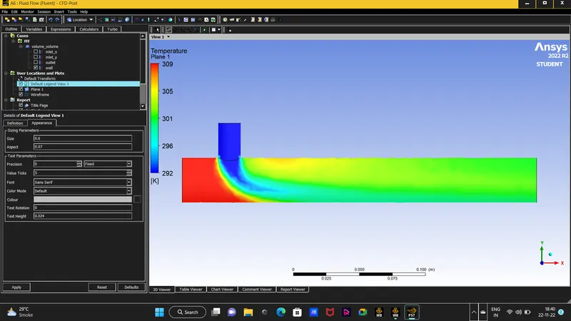 temperature plane
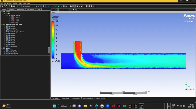 velocity plane
xy plots along and across the pipe
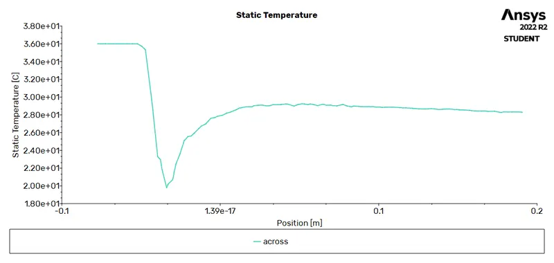 across temperatue
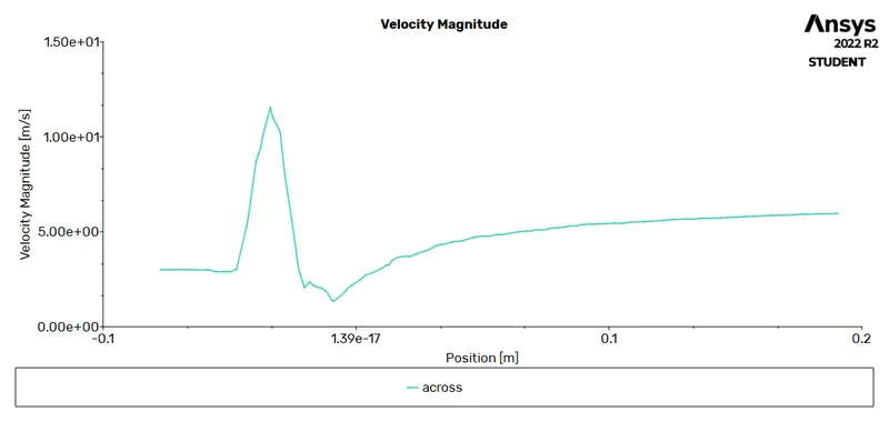 across velocity
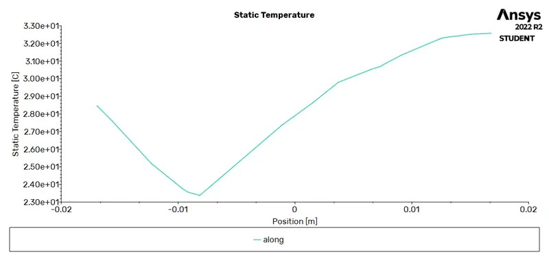
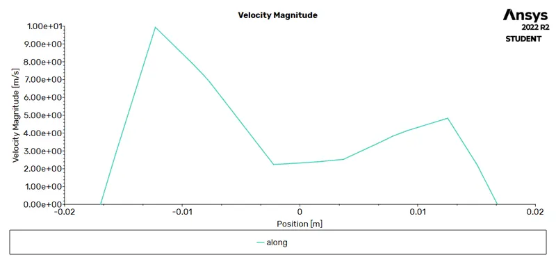 along the pipe temperature and velocity
for short tee mr = 4
for long tee mr = 2
Effects of lenght and momentum ratio:
As we learned with the grid independence that the result with the partiular short tee the result do not changes as we make the element size finer. but with that we also saw the effects of the momentum ratio that as the cold velocity inlet increases the temperature at the outlet get more mixed and the temperature of the outlet air gets little lower as we can see that in the analytical value too the Tmix value for momentum ratio of 2 is 30.02°C and for the momentum ratio of 4 the temperature value is 27.15°C.this concludes that as the momentum ratio increases the outlet temperatue will get lower. The lenght of the pipe also plays an important role as, for the short tee pipe we can see the cold and hot fluid do not mix properly as compared to the long tee for momentum ratio of 2 because for this case the velocity of the cold and hot air is same but for mixing of fluids,long tee has advantage that the cross section area of pipe is long and the fluids have more to travel as well as more time to get mixed as well.