Week 4 - CHT Analysis on Exhaust port
Aim : To simulate a Conjugate Heat Transfer analysis (CHT) on the exhaust port given.
Theory :
Heat transfer is a discipline of thermal engineering that concerns the generation , use , conversion , and exchange of thermal energy between the physical systems. heat transfer is classified into three mechanism :
1. conduction
2. convection
3. radiation
1. Conduction : Conduction is the process by which heat is transferred from the hotter end to cooler end of an object. the ability of the object to conduct heat is know as thermal conductivity , and is denoted by k. heat spontaneously flows along a temperature gradient (i.e. from hotter end to cooler end). conduction can also be defined as the transfer of heat through matter (i.e solids,liquids,gaseous) without bulk motion of the matter.
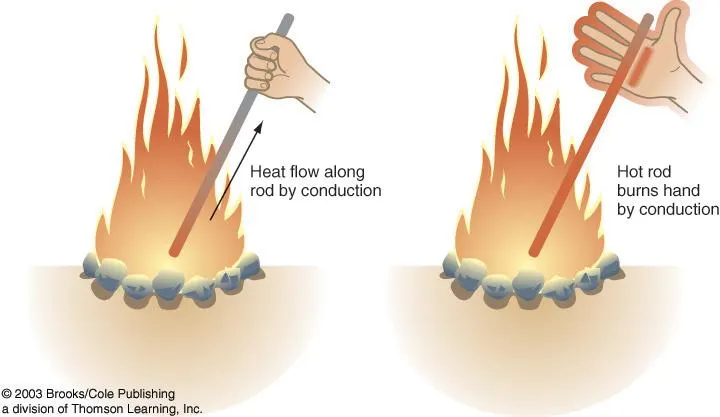
formula to calculate conduction
q = -k▼t
where q = local heat flux density
k = material conductivity
▼t = temperature gradient
2.Convection : Convection is the transfer of heat from one place to another due to the moveent of fluid. Convective heat transfer involves combined process of conductiion and advection (heat transfer by bulk fluid flow). convection is usually the dominant form of heat transfer in liquid and gases.
newton law of cooling also defines convection as the rate of heat loss of a body is proportional to the differences in the temperature between the body and its surrounding while under the effect of a brezze. the constant proportnality is the heat transfer coefficient denoted by h.
q = hA(Tsurface - tsurrounding)
q = heat tranfer
h = heat transfer coefficient W/m^3 K
A = is the area from which the heat is transfered
There are two types of convection
1. Free or Natural convection
2. Forced convection
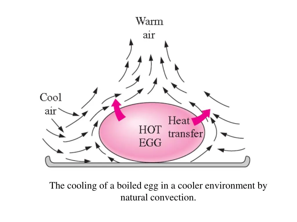
1. Free convection : it is a type of flow of motion in which the fluid motion is not generated by any external source , but by some parts of the fluid being heavier than the other parts. in most cases this leads to natural circulation , the ability of fluid system to circualte continously with gravity and possible changes in heat energy.
2.Forced convection : is a mechanism or type of tansport in which the fluid motion is generated by an external source (like pump,fan,suction etc). the mechanism is found very commonly in everyday life, including air conditioning, steam turbines and in many other machines.
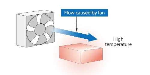 here the flow is forced by the fan to flow over the heated box.
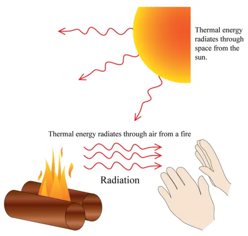
3.Radiation : heat transfer from a body with a high temperature to abody with a lower temperature, when bodies are not in contact with each other or when they are seperated in space, is called heat radiation. the radiation occurs at all temperature, with the rate of emission increasing with the temperature.
CHT Analysis : The problem of heat transfer in the presence of liquid flowing around the body was first formulated and solved as a coupled problem by Theodore L. Perelman in 1961, who also coined the term conjugate problem of heat transfer. Later T. L. Perelman, in collaboration with A.V. Luikov, developed this approach further. At that time, many other researchers started to solve simple problems using different approaches and joining the solutions for body and fluid on their interface.
The contemporary conjugate heat transfer model was developed after computers came into wide use in order to substitute the empirical relation of proportionality of heat flux to temperature difference with heat transfer coefficient which was the only tool in theoretical heat convection since the times of Newton. This model, based on a strictly mathematically stated problem, describes the heat transfer between a body and a fluid flowing over or inside it as a result of the interaction of two objects. The physical processes and solutions of the governing equations are considered separately for each object in two subdomains. Matching conditions for these solutions at the interface provide the distributions of temperature and heat flux along the body–flow interface, eliminating the need for a heat transfer coefficient. Moreover, it may be calculated using these data.
The analysis type CHT allows the simulation of heat transfer between the solid and fluid domains by exchanging thermal energy at the interfaces between them.in solids conduction usually dominates where in fluids convection usually dominates.CHT is observed in many situation example, heat sinks are optimised to combine heat transfer by conduction in the heat sink with the convection in the surrounding fluid.
The Outcome of CHT Analysis
temperature distribution analysis
heat flux rate analysis - calculation of heat transfer coefficients
temperature field analysis
evaluating variation in the temperature peaks for differnt operating conditions. and many more
Procedure to setup CHT analysis :
1.Geometry Setup
download the exhaust port geometry
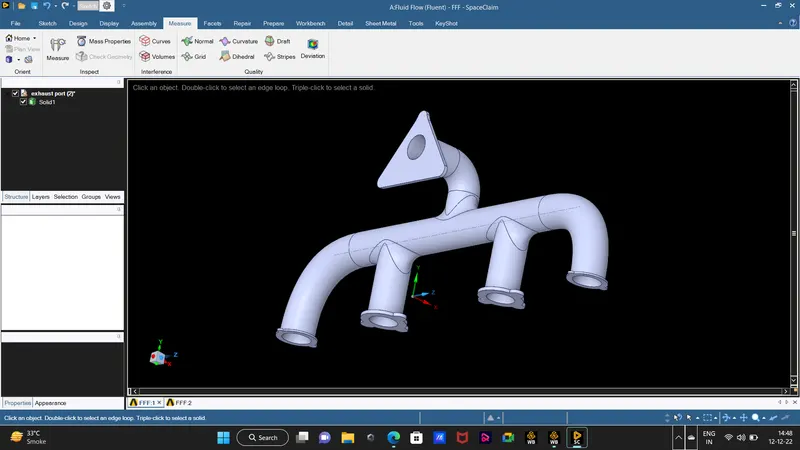
Extraction of the fluid volume
prepare> volume extraction > select the edges of the fluid volume > select ok.
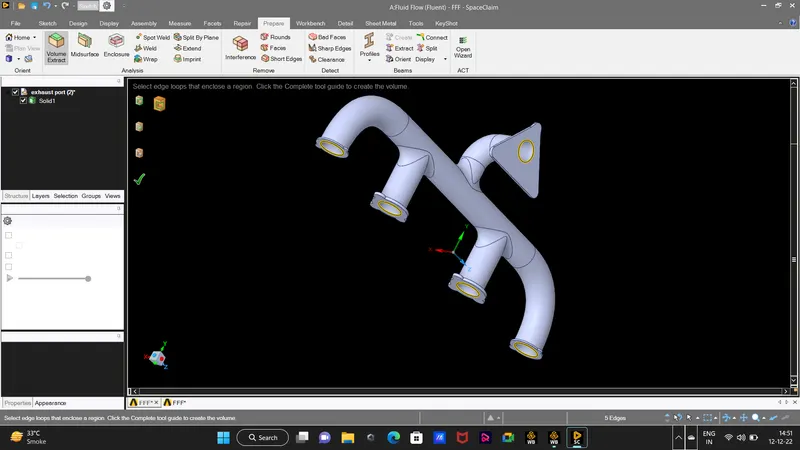
If you are not able to select the edges for the volume extraction we have to repair the geometry by deleting the duplicate entities in the geometry to do that go to
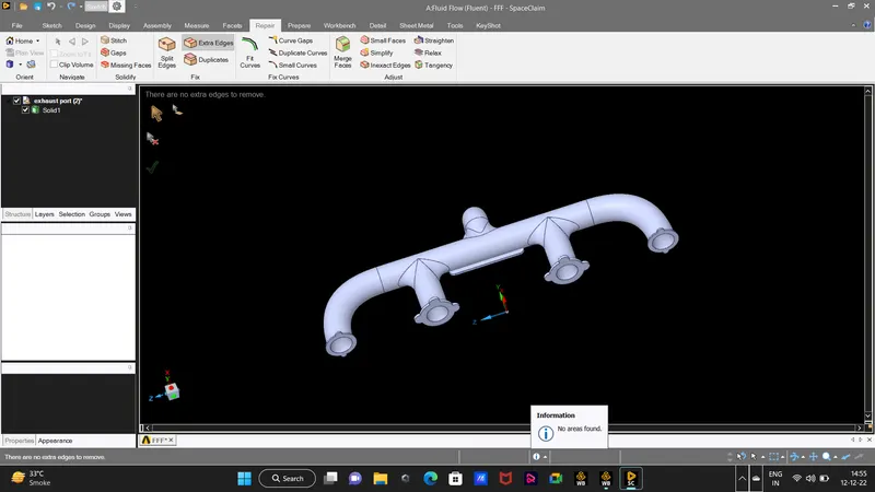
repair> Extra Edges > we will select the edges appeared in red circle > click ok; after all the duplicate entities are deleted we will recvie a messeage
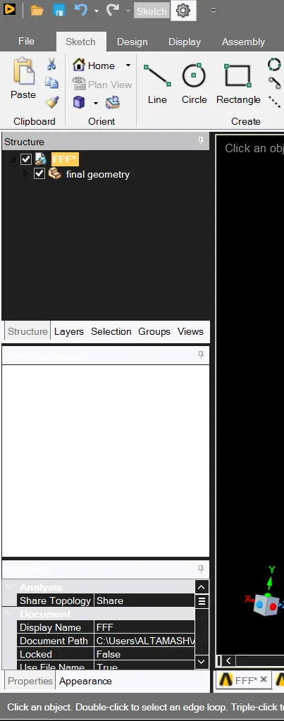
also remember to enable the share topology so that the fluid and solid geometry are shared
an important step that will create only one interface between two parts that is the solid and the fluid volume so that there is no problem in meshing.to do this step go to
Workbench > Share Prep
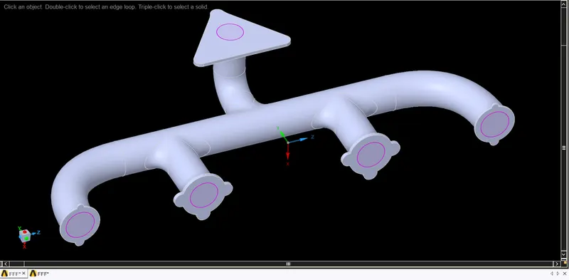 after the share prep is done then there will be pink colour edges appear as shown in the above figure. if this share prep is not done then while meshing we will look non-conformal mesh that make some physical cracks in the vertex of the fluid and solid surface
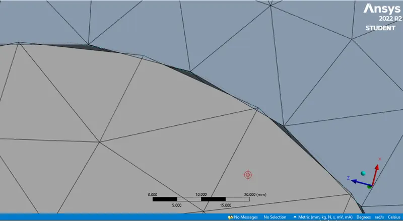 this non-conformal mesh
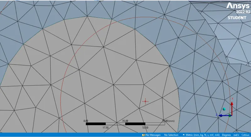 confrmal mesh as appeared ther is no cracks in the vertex and the mesh is done completely.
2. Mesh Setup :
first we will name all the boundaries of the geometry
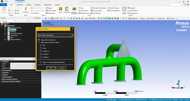 with 4 inlets, 1 outlet, the solid wall as convection-wall, and the fluid wall as inflation-layer.
first we will run a baseline mesh with number of elemnts 100mm. running a basline mesh important so that we can have an idea about how we can resolve our mesh so that we can have proper and accurate results.
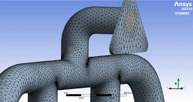
to refine the mesh
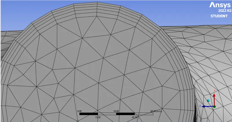
we will first create inflation layer with first layer thickness option. we selected the y+ value as 1. to calculate the first layer thickness we have to calculate
data: ρ = 1.225kg/m^3, μ = 1.789e-5, v = 5m/s, d = 0.166,
to calculate reynolds number Re = ρ*v*d / μ = 56867.6
Cf = 0.058*Re^-0.2 = 6.493e-3
τwall = 0.5*Cf*ρ*v^2 = 0.099 sheer wall stress
μt = √ τwall/ρ = 0.284 Frictional velocity
△y = y+ * μ / ρ * μt = 5.142e-5 m
= 1.542 mm is the the cell height
now to create the inflation layers
mesh > inflation layer > use named selection > seelect inflation layer named selection > selct the first layer thickness option > input the calculated height > generate mesh
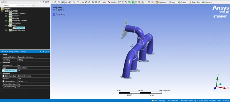
insert the body sizing and mesh the solid body
mesh insert > sizing > select the body > apply > enter the elemnt size .
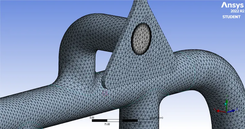 this refined mesh.
3. Fluent setup :
setting up the physics
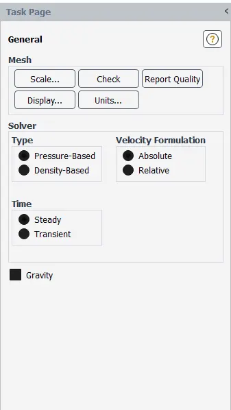
selcting the pressure based, steady , and absolute for the physics
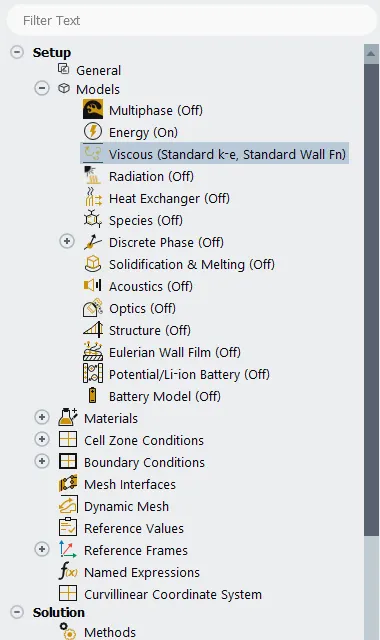
we will select the k-epsilon model with standar wall function for near wall treatment used. and also we will enable the energy as the inlet fluid will have a certain temperature.
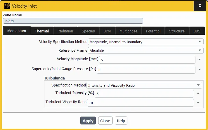
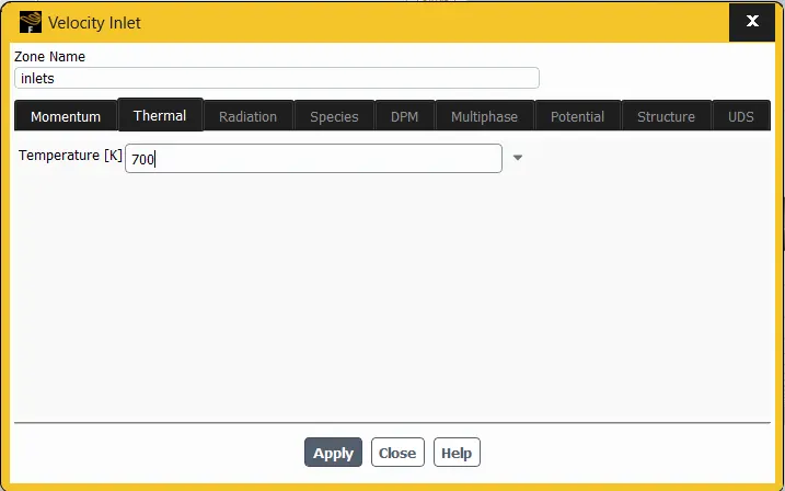
for the inlet boundary conditions we will use the inlet-velocity with 5m/s and the temperature will be 700 K
for the convection wall the boundary condition is set to convective with the heat transfer coefficient 20 W/m^2 K
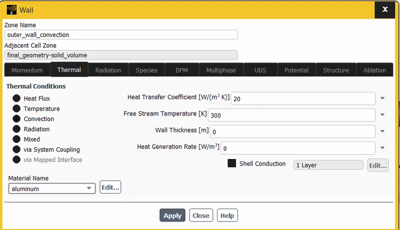
we will create temperature countor as we we will monitor the temperatre as the solution gets solved. but first we will do hybrid initialization and then go to
results > contours > name > select the boundaries > ok
now we will run the simulations and give the post process result.
Results :
for baseline mesh
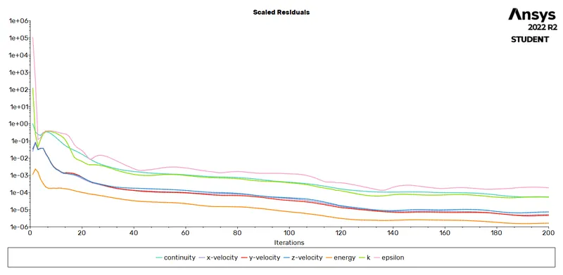 residuals.
Velocity post process result
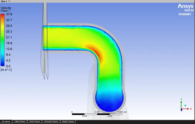 the velocity from the all the four inlets gets accumulated at the manifold which in turn increses the temperature of the fluid increses the top section which increses the velocity of the fluid and at that location we can see the maximum heat transfer from that section. the r=red section indicates the fluid velocity is highest as that we can see in the streamline result also.
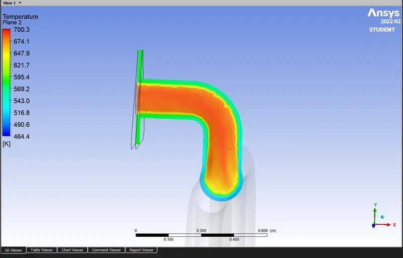
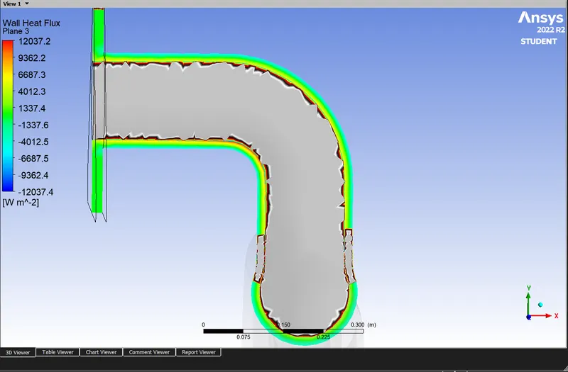 this image shows the result of heat flux or heat transfer from the fluid to the solid. the section closer to the fluid is the highest heat transfer.
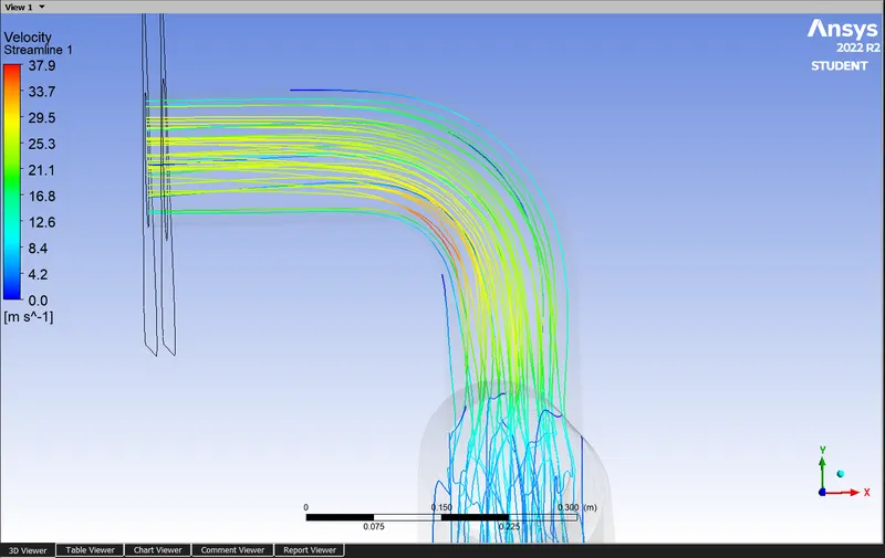 streamlines running from the inlet to outlet.
Refine mesh results :
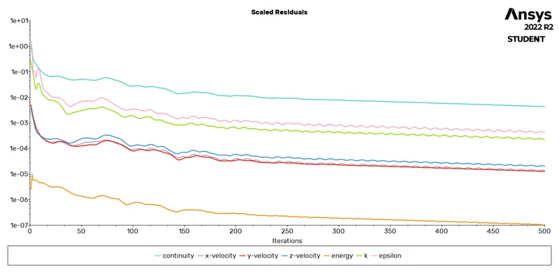
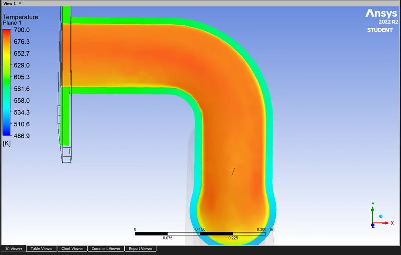
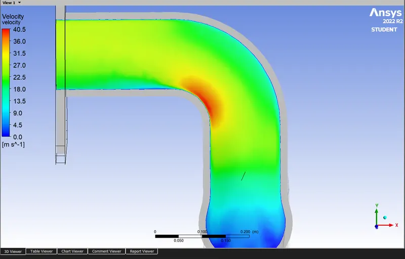
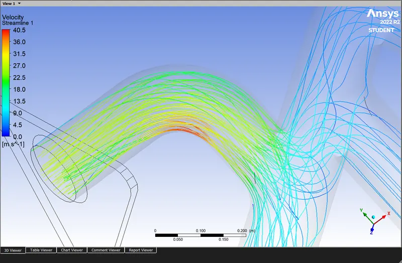
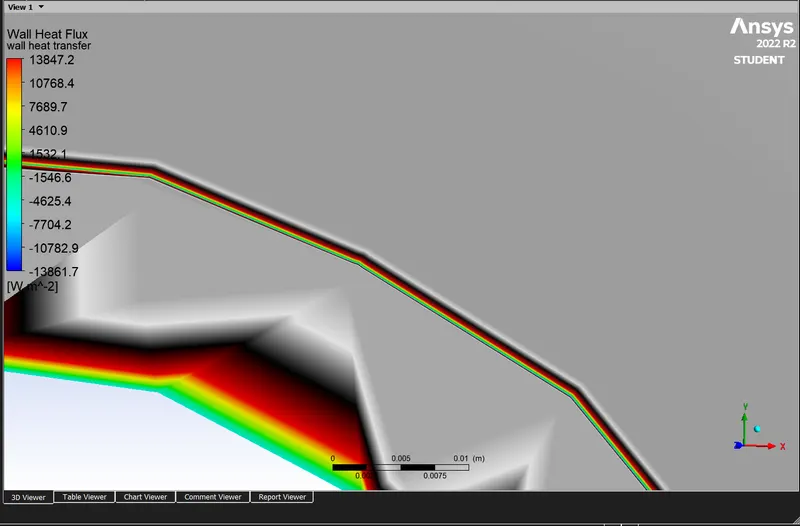 as in the refined mesh we have added the inflation layers so the layer that is visible that is the first adjacent layer to the wall and we have a very fine smooth looking heat transfer.
From our baseline mesh and the refined mesh we can see that the results are very similar and our baseline mesh is accurate to capture the heat transfer coefficient properly.
How would you verify if the HTC predictions from the simulations are right
nusselt number is the ratio of convective heat transfer to conductive heat transfer across the boundary
Nu = convective heat transfer/ condectve heat transfer = hl/k
where h = heat transfer coefficient
k = thermal conductivity of fluid
l = charachteristic lenght
relation between the reynolds and nusselt number
Nu = 0.664*Re^0.5*Pr^0.33
where Pr is Prandtl Number which is defined as ratio of kinematic viscosity by thermal diffusitivity
Pr = μCp / k
On what factors does the accuracy of the prediction depend on
from setting up the geometry we see that if the topology of the geometries are not share and the Share Prep is not achieved we can see that there were some non-conformation mesh in the setup and we was able to see the cracks in the edges shared by the solid and fluid geometry.
selection of correct turbulence model is very much important for such cases where the changes are occuring very close to the solid surface k-omega model is very suitable choice and if you are selecting k-epsilon model which is not good for near wall changes a good y+ value should predict good value.
exact heat transfer coefficient value is very cruicial. these values are expermental values. the outer or reference temperature is also important for predicting the values accurately.
correct mesh lenght is also important if the mesh is very coarse the simulation can predict the value incorrectly so a fine mesh is important. remember to always run a baseline mesh so that you can get a idea to strategically refine the mesh so that it wont increase the computational time drasttically.