Week 7 - Simulation of a 1D Supersonic nozzle flow simulation using Macormack Method
Aim : To simulate the Isentropic Flow through a Quasi 1D Subsonic-Supersonic Nozzle,for both Conservative and Non-Conservative form of Governing Equations and solve them using MacCormacks Technique.
Expected Outcome :
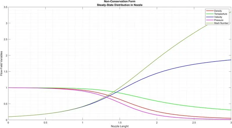
1. Steady-state distribution of primitive variables inside the nozzle
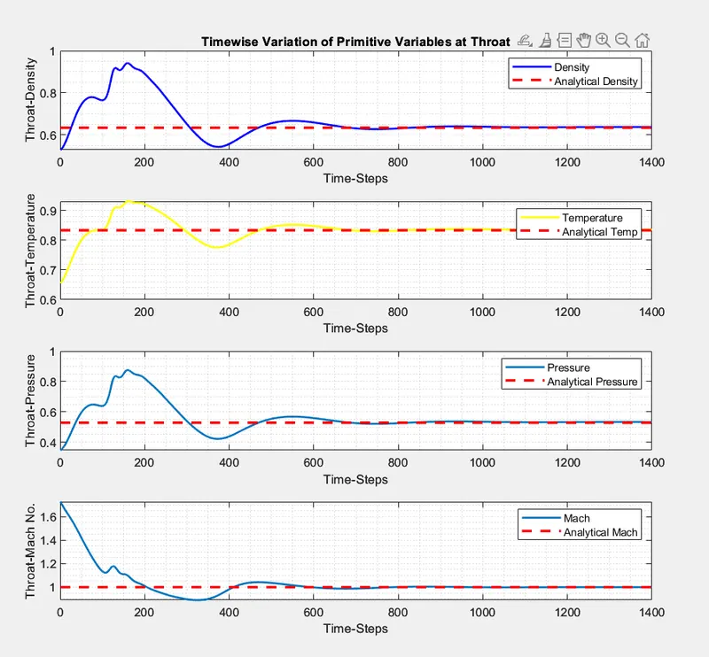
2. Time-wise variation of the primitive variables
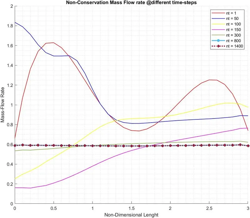
3. Variation of Mass flow rate distribution inside the nozzle at different time steps during the time-marching process
4. Comparison of Normalized mass flow rate distributions of both forms.
Theory : The Conservation and Non-Conservation form of the CFD equations are derived from Models of the Flow.Named as
- Finite Control Volume : Consider an closed volume of 'dv' ; a control surface 'ds' which bounds the volume,within a finite region of flow.
The volume can be fixed in space and the flow will paas through it or the closed surface w
ill move with the flow so there will be same fluid particles inside.
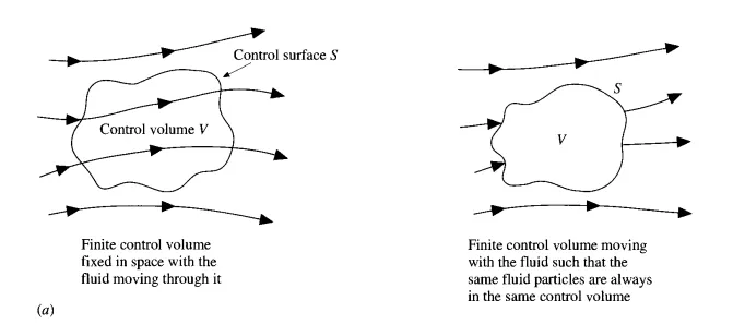
The physical equation are then applied to the fluid inside the control volume and the fluid crossing the control surface.
The equations obtained from the Finite Control Volume Fixed in Space is called Conservation Form and the Equations obtained from the Finite Control Volume moving with the fluid are called Non-Conservation form of the governing equations.
MACCORMACKS TECHNIQUE :
MacCormacks Technique is the variant and simpler version of the Lax-Wendroff Technique.Both of the techniques are finite differenc , second-order-accurate in both space and time.
However MacCormacks tech is very easy for writting the code as we dont have to compute the mixed derivatives terms that are generated in the Lax-Wendroff Tech while computing Taylor Series for the flow-field variable.The algebra of the MacCormacks is not very lenghty like the latter.
The MacCormacks method for a variable is obtained by
`phi_(i)^(t+dt) = phi_(i)^(t) + ((delphi)/(delt))_(av)*dt` ------(1)
where `((delphi)/(delt))_(av)`is a representative mean value of the `(delphi)/(delt)` between t and t+dt.That is taking a mean average of the variable at old time step and the new time steps.
The Average term is calculated by Predictor -Corrector philosophy,
Predictor Step : The spatial derivatives of the function (`phi`) are replaces with the forward difference scheme
`((delphi)/(delt))_i^t = ((phi_(i+1)^t + phi_i^t)/dx )` ----------(2)
Now we will obtain the predicted values from eq(1),from the first two terms of the Taylor Series
`barphi_i^(t+dt) = phi_i^t + ((delphi)/(delt))_i^t * dt` ------(3)
the barred values will readily obtained as the right hand side of the eq(3) is at time t and the time term will be obtained form eq(2).
Corrector Step : We first obtain the time derivative value of the function at t+dt (as the Time Average Term is arhtematic mean at t and t+dt steps), by substituting the the barred values for the function (`phi`) and replacing the spatail derivative terms with rearward differencing scheme
`((delbarphi)/(delt))_i^(t+dt) = ((barphi_(i+1)^(t+dt) + barphi_i^(t+dt))/dx )` -------------(4)
Now the Average time derivative term will be calculated by taking the arthematic mean of equation (1) and (3),
`((delphi)/(delt))_(av) = 1/2*(((delphi)/(delt))_i^t + ((delphi)/(delt))_i^(t+dt))` --------------(5)
and finally substitung equation(5) in the eq(1).
The value of the function `phi` at grid point i,at time d+dt is yielded by means of MacCormacks Technique.Here we are sparred with large number of calculations as mentioned in the Lax-Wendroff Technique.
This procedure will be use to solve our problem is Nozzle flow.
- Solution Setup : The conservation and non-sonservation form of the governing equation is given as,
Nozzles Flows,the flow field variables are frequently expressed in terms of nondimensional varibles.
Defining the nondimensional variables:
Nondimensional Temperature:`T' = T/T_0`
Nondimensional Density:`rho' = rho/rho_0`
Nondimensional Lenght:`x' = x/L`
Nondimensional Velocity:`v' = V/V_0`
Nondimensional Time:`t' = t/(L/a_0)`
Nondimensional Area:`A' = A/(A**)`
The mention conservation and non conservation form are expressd as nondimensional terms and for sake of simplicity will drop the prime sign
- Non-Conservation Form Governing Equations:
Continuity Equation : `(delrho)/(delt) = -rho*(delv)/(delx) - rho*v*(delln(A))/(delx) - v*(delrho)/(delx)`
Momentum Equation : `(delv)/(delt ) = -v*(delv)/(delx)-(1/gamma)*((delT)/(delx) + T/rho * (delrho)/(delx))`
Energy Equation : `(delT)/(delt) = -v*(delT)/(delx)-(gamma-1)*T*((delv)/(delx)+v*(delln(A))/(delx))`
- Conservation Form of Governing Equation
Continuity Equation : `(delrhoA)/(delt) + (delrhoAv)/(delx)`
Momentum Equation : `(delrhoAv)/(delt) + (del[rhoAv^2 + (1/gamma)*rhoA])/(delx) = 1/gamma*p*(delA)/(delx)`
Energy Equation : `(del[rho*(e/(gamma-1)+gamma/2*v^2)*A])/(delt) + (del[rho(e/(gamma-1)+gamma/2*v^2)*v*A+p*A*V])/(delx)`
writing the non-conservation equations in generic form.
u be solution vector , f be flux vector and J be source term
Solution Vectors
u1 = `rho*A`
u2 = `rho*A*v`
u3 = `rho*(e/(gamma-1)+gamma/2*v^2)*A`
Flux Vectors
f1 = `rho*A*v`
f2 = `rhoAv^2 + 1/gammapA`
f3 = `rho*(e/(gamma-1)+gamma/2*v^2)vA+pAv`
Source Term
J = `1/gamma*p*(delA)/(delx)`
therefore,the equations can be written as
`(delu1)/(delt) = -(delf1)/(delx)`
`(delu2)/(delt) = -(delf2)/(delx) + J`
`(delu3)/(delt) = -(delf3)/(delx)`
From the above equations of the conservation form the dependent variables for which we directly obtain the values are not primitive variables,therefore to calculate the variable we will decode the solution vectors,
`rho = (u1)/A`
`v = (u2)/(u1)`
`T = (gamma-1)*((u3)/(u1)-gamma/2*v^2)`
Refering to John.D.Anderson Book
writting the flux vectors in terms of primitive variable blow up the solution after s=certain time steps.So expressing flux vectors f1,f2 and f3 in terms of u1,u2 and u3 and avoid the use of primitive variables.
Therefore the flux vectors in terms of u1,u2 and u3 are given as
f1 = u2
`f2 = (u2)^2/(u1) + (gamma-1)/gamma*(u3 - gamma/2*((u2)/(u1))^2)`
`f3 = gamma*(u2*u3)/(u1) - (gamma*(gamma-1))/2*(u3)^2/(u1)^2`
`J = (gamma-1)/gamma*(u3-gamma/2*(u2)^2/(u1)*(delln(A))/(delx))`
Time Step Calculation : To avoid 'artifical time warp', we will calculate the time step at every node and then take the minimum value of the time step to calculate at every time step in the time marching solution.
`dt = min(C*dx/(T^(1/2)+v))`
- Nozzle Shape : Nozzle shape is defined as
`A = 1+2.2*(x-1.5)^2` `0<=x<=3`
- Initial Conditions for Both form
- Non-Conservation form Initial Conditions of flow-field variable
`rho = 1-0.3146*x` for t = 0
`T = 1-0.2314*x`
`v = (0.1+1.09*x)*T^(1/2)`
- Conservation form Initial Conditions of flow-field variable
`rho = 1` }`0<=x<=0.5`
`T = 1` }
`rho = 1-0.366*(x-0.5)`
`T = 1-0.167*(x-0.5)` for `0.5<=x<=1.5`
`rho = 0.634-0.3879*(x-1.5)`
`T = 0.833-0.3507*(x-1.5)` for`1.5<=x<=3.5`
- Boundary Conditions :
- Non-Conservation form
Subsonic Inlet
`rho(1) = 1`
T(1) = 1
v(1) = 2*v(2)-v(3)
Supersonic Outflow
`rho(n) = 2*rho(n-1)-rho(n-2)`
T(n) = 2*T(n-1)-T(n-2)
v(n) = 2*v(n-1)-v(n-2)
- Non-conservative form
Subsonic Inlet
`u1(1) = rho(1)*A(1)`
u2(1) = 2*u2(2) - u2(3)
v(1) = u2(1)/u1(1);
u3(1) = u1(1)*(t(1)/(gamma-1)+(gamma/2)*v(1)^2);
Supersonic Outflow
u1(n) = 2*u1(n-1)-u1(n-2)
u2(n) = 2*u2(n-1)-u2(n-2)
u3(n) = 2*u3(n-1)-u3(n-2)
Now we will setup the numerical solution for the Conserve and Non-Conserve form and evaluate the results.
- Matlab Code :
- Main Code :
%Sub-sonic Supersonic 1-D Nozzle flow main program
clear all
close all
clc

%Inputs
n = 31;
x = linspace(0,3,n);
dx = x(2) - x(1);
gamma = 1.4;
C = 0.5;

nt = 1400;

%Nozzle profile
a = 1+2.2*(x-1.5).^2;

throat = find(a==1);            %To find index of a that corresponds to value 1

%Analytical Values of Flow-Field Variables
% rho_ana = 0.634;
% pressure_ana = 0.528;
% M_ana = 1;
% t_ana = 0.833;

for y = 1:n
    mfr_ana(y) = 0.579;
end


%Calling the function
tic
[mfr,mfr_thr] = N_C(n,x,dx,gamma,a,C,throat,nt);
NConserv_Cmpt_time = toc

tic
[mfr_c,mfr_thr_c] = c_form(n,x,dx,gamma,a,C,throat,nt);
Conserv_Cmpt_time = toc

figure(7)
plot(x,mfr,LineWidth=1.5,Color='b')
hold on
plot(x,mfr_c,Color='m',linewidth=1.5)
plot(x,mfr_ana,LineWidth=2,Color='r')
title('Mass Flow Rate of Different Form of equations')
legend('Non-Conservation','Conservation','Analytical')
grid on- function for Non_Conservation Form :
%Function for Non-Conservation Form

function [mfr,mfr_thr] = N_C (n,x,dx,gamma,a,C,throat,nt)
%Intial Profiles
rho = 1-0.3146*x;
t = 1-0.2314*x;
v = (0.1+1.09*x).*t.^0.5;

A = (t.^(1/2));

%MacCormacks Technique

for k = 1:nt
%Time step calculation
    dt = min(C*(dx ./((A)+v)));

    %updating old values
    rho_old = rho;
    v_old = v;
    t_old = t;
    mfr_old = rho_old.*v_old.*a;

    % predictor method
    for j = 2:n-1
        dvdx = (v(j+1)-v(j))/dx;
        drhodx = (rho(j+1)-rho(j))/dx;
        dtdx = (t(j+1)-t(j))/dx;
        dlogadx = (log(a(j+1))-log(a(j)))/dx;

        % Continuity equation
        drhodt_p(j) = -rho(j)*dvdx - rho(j)*v(j)*dlogadx - v(j)*drhodx;

        % Momentum eqn
        dvdt_p(j) = -v(j)*dvdx - (1/gamma)*(dtdx + (t(j)/rho(j))*drhodx);

        % Energy eqn
        dtdt_p(j) = -v(j)*dtdx - (gamma - 1)*t(j)*(dvdx + v(j)*dlogadx);

        % Soln update
        rho(j) = rho(j) + drhodt_p(j)*dt;
        v(j) = v(j) + dvdt_p(j)*dt;
        t(j) = t(j) + dtdt_p(j)*dt;
    end

    % Corrector method
    for j = 2:n-1
        dvdx = (v(j)-v(j-1))/dx;
        drhodx = (rho(j)-rho(j-1))/dx;
        dtdx = (t(j)-t(j-1))/dx;
        dlogadx = (log(a(j))-log(a(j-1)))/dx;

        % Continuity equation
        drhodt_c(j) = -rho(j)*dvdx - rho(j)*v(j)*dlogadx - v(j)*drhodx;

        % Momentum eqn
        dvdt_c(j) = -v(j)*dvdx - (1/gamma)*(dtdx + (t(j)/rho(j))*drhodx);

        % Energy eqn
        dtdt_c(j) = -v(j)*dtdx - (gamma - 1)*t(j)*(dvdx + v(j)*dlogadx);

    end

    drhodt_av = 0.5*(drhodt_p + drhodt_c);
    dtdt_av = 0.5*(dtdt_p + dtdt_c);
    dvdt_av = 0.5*(dvdt_p + dvdt_c);

    for i = 2:n-1
        rho(i) = rho_old(i) + drhodt_av(i)*dt;
        t(i) = t_old(i) + dtdt_av(i)*dt;
        v(i) = v_old(i) + dvdt_av(i)*dt;
    end

%B.C
%Inlet
rho(1) = 1;
t(1) = 1;
v(1) = 2*v(2) - v(3);

%Outlet
rho(n) = 2*rho(n-1) - rho(n-2);
t(n) = 2*t(n-1) - t(n-2);
v(n) = 2*v(n-1) - v(n-2);

%Calculating Other Flow-Field Variables
mfr = rho.*v.*a;                  %Mass Flow Rate
prssr = rho.*t;                   %Pressusre
mach = v./(t.^(1/2));             %Mach Number

%Analytical solution
rho_ana(k) = 0.634;
pressure_ana(k) = 0.528;
M_ana(k) = 1;
t_ana(k) = 0.833;

%Flow Field Varaibles at Throat
rho_thr(k) = rho(throat);
v_thr(k) = v(throat);
t_thr(k) = t(throat);
prssr_thr(k) =  prssr(throat);
mfr_thr(k) = mfr(throat);
mach_thr(k) = mach(throat);

%PLotting the Mass Flow Rate For different Time-steps
figure(1)
hold on
if k == 1
    plot(x,mfr,'r','LineWidth',1)
elseif k == 50
    plot(x,mfr,'b','linewidth',1)
elseif k == 100
    plot(x,mfr,'y','linewidth',1)
elseif k == 150
    plot(x,mfr,'m','linewidth',1)
elseif k == 300
    plot(x,mfr,'LineWidth',1)
elseif k == 800
    plot(x,mfr,'LineWidth',2,'Marker','*',MarkerFaceColor='auto')
elseif k == 1400
    plot(x,mfr,'LineWidth',2.5,LineStyle=':',Marker='+')
    xlabel('Non-Dimensional Lenght')
    ylabel('Mass-Flow Rate')
    legend('nt = 1','nt = 50','nt = 100','nt = 150','nt = 300','nt = 800','nt = 1400')
    title('Non-Conservation Mass Flow rate @different time-steps')
    grid minor
end

end

X = linspace(1,nt,nt);
figure(2)
%Timewise Variation of Primitive Variables
subplot(4,1,1)
plot(X,rho_thr,'b','linewidth',1.5)
hold on
plot(X,rho_ana,'r',LineWidth=2,LineStyle='--')
xlabel('Time-Steps')
ylabel('Throat-Density')
title('Timewise Variation of Primitive Variables at Throat')
legend('Density','Analytical Density')
grid minor

subplot(4,1,2)
plot(X,t_thr,'y','linewidth',1.5)
hold on
plot(X,t_ana,'r',LineWidth=2,LineStyle='--')
xlabel('Time-Steps')
ylabel('Throat-Temperature')
legend('Temperature','Analytical Temp')
grid minor

subplot(4,1,3)
plot(X,prssr_thr,'linewidth',1.5)
hold on
plot(X,pressure_ana,'r',LineWidth=2,LineStyle='--')
xlabel('Time-Steps')
ylabel('Throat-Pressure')
legend('Pressure','Analytical Pressure')
grid minor

subplot(4,1,4)
plot(X,mach_thr,'linewidth',1.5)
hold on
plot(X,M_ana,'r',LineWidth=2,LineStyle='--')
xlabel('Time-Steps')
ylabel('Throat-Mach No.')
legend('Mach','Analytical Mach')
grid minor

figure(3)
%Steady-State Distribution of variable in Nozzle
plot(x,rho,'r','LineWidth',1.5)
hold on
plot(x,t,'g','LineWidth',1.5)
plot(x,v,'b','LineWidth',1.5)
plot(x,prssr,'m','LineWidth',1.5)
plot(x,mach,'LineWidth',1.5)
hold off
xlabel('Nozzle Lenght')
ylabel('Flow-Field Variables')
title({['Non-Conservation Form'];['Steady-State Distribution in Nozzle']})
legend('Density','Tempearture','Velocity','Pressure','Mach Number')
grid minor

end- function for Conservation Form :
% function for Conservation Form
function [mfr_c,mfr_thr_c] = c_form(n,x,dx,gamma,a,C,throat,nt)

% Intialising the profiles
for q = 1:n
    if (x(q) >= 0 && x(q) <= 0.5)
        rho_c(q) = 1;
        t_c(q) = 1;
    elseif (x(q) >= 0.5 && x(q) <= 1.5)
        rho_c(q) = 1-0.366*(x(q)-0.5);
        t_c(q) = 1-0.167*(x(q)-0.5);
    elseif (x(q) >= 1.5 && x(q) <= 3.5)
        rho_c(q) = 0.634-0.387*(x(q)-1.5);
        t_c(q) = 0.833-0.3507*(x(q)-1.5);
    end
end


A_c = t_c.^(1/2); %Term in the time-step control

% Intial velocity profile
v_c = 0.59./(rho_c.*a);
p_c = rho_c.*t_c;              %Pressure Initial profile

% Intialising the solution vector
u1 = rho_c.*a;
u2 = rho_c.*v_c.*a;
u3 = rho_c.*(t_c./(gamma-1) + (gamma/2).*v_c.^2).*a;

% A_c = t_c.^(1/2);

%Initiating the MacCormacks Technique
for k = 1:nt
    %Calculating the Time-Step
    dt = C*(dx./(A_c+v_c));
    dt = min(dt);

    %retaing old values
    u1_old = u1;
    u2_old = u2;
    u3_old = u3;

    %Flux terms
    f1 = u2;
    f2 = (u2.^2)./(u1) + ((gamma-1)/gamma) * (((u3-(gamma/2)*((u2.^2))./u1)));
    f3 = gamma*(u2.*u3)./u1 - (gamma*(gamma-1)/2) * (u2.^3)./(u1.^2);

    %Predictor Step
    for j = 2:n-1
        df1dx = (f1(j+1)-f1(j))/dx;
        df2dx = (f2(j+1)-f2(j))/dx;
        df3dx = (f3(j+1)-f3(j))/dx;
        source = (1/gamma) * rho_c(j) * t_c(j) * ((a(j+1)-a(j))/dx);

        %Continuity Equation
        du1dt_p(j) = -df1dx;

        %Momentum Equation
        du2dt_p(j) = -df2dx + source;

        %Energy Equation
        du3dt_p(j) = -df3dx;

        %Solution Update
        u1(j) = u1_old(j) + du1dt_p(j)*dt;
        u2(j) = u2_old(j) + du2dt_p(j)*dt;
        u3(j) = u3_old(j) + du3dt_p(j)*dt;

    end
    %Predicted Primitive Values
    rho_c = u1./a;
    v_c = u2./u1;
    t_c = (gamma-1) * (u3./u1 - (gamma/2)*(v_c.^2));

    %Updating the flux terms(for corrector step)
    f1 = u2;
    f2 = (u2.^2)./(u1) + ((gamma-1)/gamma) * (((u3-(gamma/2)*((u2.^2))./u1)));
    f3 = (gamma*(u2.*u3)./u1) - (gamma*(gamma-1)/2) * (u2.^3)./(u1.^2);

    %Corrector Step
    for j = 2:n-1
        df1dx = (f1(j)-f1(j-1))/dx;
        df2dx = (f2(j)-f2(j-1))/dx;
        df3dx = (f3(j)-f3(j-1))/dx;
        source = (1/gamma) * rho_c(j) * t_c(j) * ((a(j)-a(j-1))/dx);

        %Continuity Equation
        du1dt_cr(j) = -df1dx;

        %Momentum Equation
        du2dt_cr(j) = -df2dx + source;

        %Energy Equation
        du3dt_cr(j) = -df3dx;
    end

    %Avearge Time Derivative Term
    du1dt_av = 0.5*(du1dt_p + du1dt_cr);
    du2dt_av = 0.5*(du2dt_p + du2dt_cr);
    du3dt_av = 0.5*(du3dt_p + du3dt_cr);

    %Calculating Primitive Variable for next time-step
    for z = 2:n-1
        u1(z) = u1_old(z) + du1dt_av(z) * dt;
        u2(z) = u2_old(z) + du2dt_av(z) * dt;
        u3(z) = u3_old(z) + du3dt_av(z) * dt;
    end

%Applying thr B.C
%Inlet B.C
    rho_c(1) = 1;
    t_c(1) = 1;
    u1(1) = rho_c(1)*a(1);
    u2(1) = 2*u2(2) - u2(3);
    v_c(1) = u2(1)/u1(1);
    u3(1) = u1(1)*(t_c(1)/(gamma-1)+(gamma/2)*v_c(1)^2);

    % Outlet B.C
    u1(n) = 2*u1(n-1) - u1(n-2);
    u2(n) = 2*u2(n-1) - u2(n-2);
    u3(n) = 2*u3(n-1) - u3(n-2);

%Calculting the corrected primitive values
rho_c = u1./a;
v_c = u2./u1;
t = (gamma-1)*(u3./u1-(gamma/2)*(v_c.^2));

M_c = v_c./(t_c.^0.5);
p_c = rho_c.*t_c;
mfr_c = rho_c.*v_c.*a;

% Analytical solution
rho_ana(k) = 0.634;
pressure_ana(k) = 0.528;
M_ana(k) = 1;
t_ana(k) = 0.833;

%Flow Field Varaibles at Throat
rho_c_thr(k) = rho_c(throat);
v_c_thr(k) = v_c(throat);
t_c_thr(k) = t_c(throat);
prssr_c_thr(k) =  p_c(throat);
mfr_thr_c(k) = mfr_c(throat);
mach_c_thr(k) = M_c(throat);

%PLotting the Mass Flow Rate For different Time-steps
figure(4)
hold on
if k == 1
    plot(x,mfr_c,'r','LineWidth',1.5,LineStyle='-')
elseif k == 50
    plot(x,mfr_c,'b','linewidth',1.5)
elseif k == 100
    plot(x,mfr_c,'linewidth',1.5)
elseif k == 150
    plot(x,mfr_c,'linewidth',1.5)
elseif k == 200
    plot(x,mfr_c,'LineWidth',1.5,'Color','m',Marker='+')
elseif k == 700
    plot(x,mfr_c,'LineWidth',2,'Marker','*',MarkerFaceColor='auto')
elseif k == 1400
    plot(x,mfr_c,'LineWidth',2.5,LineStyle=':',Marker='+')
    xlabel('Non-Dimensional Lenght')
    ylabel('Mass-Flow Rate')
    legend('nt = 1','nt = 50','nt  = 100','nt = 150','nt = 200','nt = 700','nt = 1400')
    title({['Conservation Form'];['Mass Flow Rate Different Time-steps']})
    grid minor

end

end

X = linspace(1,nt,nt);
figure(5)
%Timewise Variation of Primitive Variables
subplot(4,1,1)
plot(X,rho_c_thr,'b','linewidth',1.5)
hold on
plot(X,rho_ana,'r',LineWidth=2,LineStyle='--')
xlabel('Time-Steps')
ylabel('Throat-Density')
title({['Conservation Form'];['Timewise Variation of Primitive Variables at Throat']})
legend('Density','Analytical Density')
grid minor

subplot(4,1,2)
plot(X,t_c_thr,'y','linewidth',1.5)
hold on
plot(X,t_ana,'r',LineWidth=2,LineStyle='--')
xlabel('Time-Steps')
ylabel('Throat-Temperature')
legend('Temperature','Analytical Temp')
grid minor

subplot(4,1,3)
plot(X,prssr_c_thr,'linewidth',1.5)
hold on
plot(X,pressure_ana,'r',LineWidth=2,LineStyle='--')
xlabel('Time-Steps')
ylabel('Throat-Pressure')
legend('Pressure','Analytical Pressure')
grid minor

subplot(4,1,4)
plot(X,mach_c_thr,'linewidth',1.5)
hold on
plot(X,M_ana,'r',LineWidth=2,LineStyle='--')
xlabel('Time-Steps')
ylabel('Throat-Mach No.')
legend('Mach','Analytical Mach')
grid minor

figure(6)
%Steady-State Distribution of variable in Nozzle Conservation Form
plot(x,rho_c,'r','LineWidth',1.5)
hold on
plot(x,t_c,'g','LineWidth',1.5)
plot(x,v_c,'b','LineWidth',1.5)
plot(x,p_c,'m','LineWidth',1.5)
plot(x,M_c,'LineWidth',1.5)
hold off
xlabel('Nozzle Lenght')
ylabel('Flow-Field Variables')
title({['Conservation Form'];['Steady-State Distribution in Nozzle']})
legend('Density','Tempearture','Velocity','Pressure','Mach Number')
grid minor

end
Code Explanation :
- The Code is written for conservation and non-conservation form in the form of function and then these functions are called in the main program.
- In the main program inputs are initialised which will be used as function inputs as well.The inputs variables are,Number of nodes(n),mesh (x),size of mesh(dx),Courant Number(C) and number of time-steps(nt).The throat variable stores the index value of area(a) which is 1.The 'find' is an in-built matlab function that will find which index does 'a' is 1.Nozzle profile is defined as (a).
- In the main code we have also mentioned the Mass Flow Rate Analytical Value so that we can compare the mass flow rate of all three forms.As it is shown in the plot section in the main code.
- Writting the function for both forms.We have only taken mass flow rate through the nozzle and mass flow rate at throat section as an output for both of the functions.
- In the function for both of the forms first we have initialized the initial profiles of the primitive variables as mentioned in the John.Anderson textbook.For the Conservation form we also have to initialize the Solution Vectors as mentioned in the theory.
- As intialization of all variables are done we will start our computation of the MacCormacks Technique,by first initializing the time loop.Inside the loop first we will calculate the minimum time-step value calculated for every node.Also we will reatain values of the variables at former time-step.
- After that we will start computing the first step of Maccormacks tech by calculating the Prediction Values of the variables for all the Internal Nodes,by dicretizing all spatial derivatives terms with the Forward Differencing Scheme.Inside that spatial loop we will update our primitive variable solution that is calculating the barred values(`barphi^(t+dt)`) at time dt.
- Then those updated vales will be used to calculate the Corrector Step values at time step dt,similarly as done for the predictor step for all the internal nodes.The only change in this step will be that all the spatial derivative terms will be calculated by discretizing by Backward Differencing Scheme.
- As we have computed values for Predictor Step at time step(t) and Corrector Step at time step(t+dt).Now we will compute the Average Time Derivative Term for all the respective flow field variables by taking the arthematic mean of the predictor and corrector step.
- Finally we will conclude the last step by calculating the value of the Primitive variable at the next time-step.And with this step the calculation of the flow field variable for a single time step is completed.This steps will continue for the Number of Time-Steps mentioned in the time loop.For our case the solution is seems to converges around 800 time steps.The values of the primitive variables at throat at all time steps are also saved by taking the index value as saved in the throat variable.
- Inside the time loop we will initialize the Boundary Conditions for the respective forms as mentioned.Two values will be fixed and one value will float.The value of the velocity is set to afloat and B.C condition is calculated by extrpolatting the values at node number 2 and 3.
- Also then we will compute our results,first by plotting the Mass Flow Rate at different time steps for both forms of equations.This is done inside the time loop using the index as used in the time loop.Here to plot at different time step we will use the 'if' conditional statements to plot for differnet time-steps.
- Outside the time loop we will plot the Timewise Variation of variable at throat and comparing it with the Analytical values of the primitive variables at throat.
- All the results are plotted.
Results :
- Plots and Results for Non-Conservation Form :
(a).Steady-State Distribution of Variables in Nozzle
(b).Time-Variation of the primitive variables at throat.
(c).Mass Flow Rate at different Time-steps.
From the result(b) the largest changes takes place at early time-steps after which the variables reaches steady state.The chnages in the latter time steps are very small and the numerical solution converges to the exact solution after 800 time steps.
From the result (c) from the plot it is seen that the values of the mass flow rate changes considerably after 50 time steps, same goes for 100 time steps.The mass flow rate chnages inside the nozzle due to variation of the primitive variables.But after 800 time steps the mass flow dosent change and a steady state of mass flow rate is achieved that is shown by blue color line with 0 marker.
- Grid Independency Study
| Variables values at thorat | |||||
| `(rho**)/rho_0` | `(t**)/t_0` | `(p**)/p_0` | Mach Number | ||
| Case 1. | 31 grid points | 0.638 | 0.836 | 0.534 | 0.999 |
| Case 2. | 61 grid points | 0.638 | 0.835 | 0.532 | 0.999 |
| Exact Solution | 0.634 | 0.833 | 0.528 | 1.000 |
From the above table the results does not changes when the grid points are doubled or the dx is reduced to half hence running the simulation for 31 grid points will give an accurate results too.So we can run the simulation for 31 grid points for Conservation form.
- Plots and Results for Conservation Form :
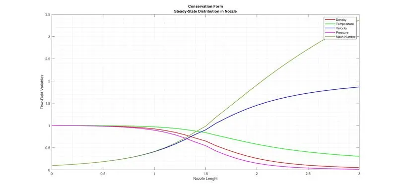
(d).Steady-State Distribution of Variables in Nozzle
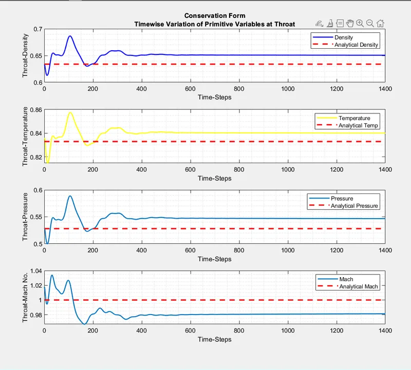
(e).Time-Variation of the primitive variables at throat.
(f).Mass Flow Rate at different Time-steps.
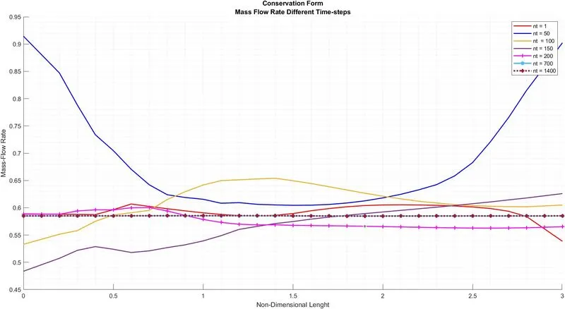
From the plot (e) the variation in the mass flow rate after 100 time steps becomes less rigours as vice-versa seen for the non-conservation form.After 700 time steps the changes are cannot be seen for the conservation form that concludes it reaches steady state.
- Comparison of Steady-State results,Conservation v/s Non-Conservation
| `(rho**)/rho_0` | `(t**)/t_0` | `(p**)/p_0` | Mach Number | |
| Exact Solution | 0.634 | 0.833 | 0.528 | 1.000 |
Non_conserve (31 grid points) | 0.638 | 0.836 | 0.534 | 0.999 |
Non_conserve (61 grid points) | 0.637 | 0.835 | 0.532 | 0.999 |
Conservative (31 grid points) | 0.650 | 0.840 | 0.546 | 0.981 |
Conservative (61 grid points) | 0.638 | 0.835 | 0.533 | 0.999 |
the result of the above table agrees with the values obtained in the John.D.Anderson textbook.
- Mass Flow Rate of Conservation v/s Non-Conserve v/s Analytical Plot :
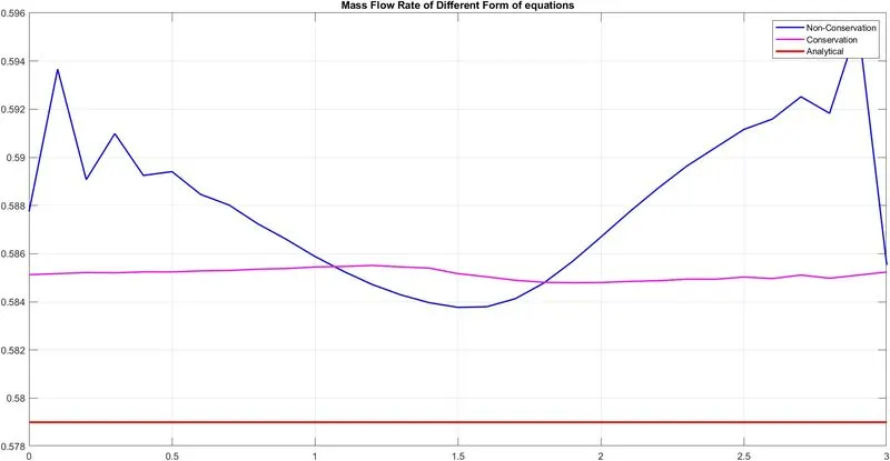
(g) for 31 grid points.
(h) 61 grid points
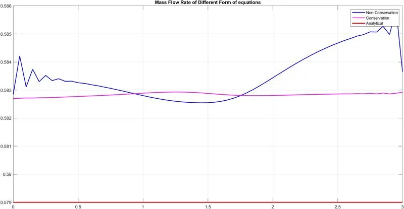
From the above results we can say that the mass flow rate obtained from the conservation form is much more closer to analytical solution than the profile obtained from non-conservation form.
Conclusion :
- The Conservation form yields a better mass flow distribution.
- Both form gives an accurate results.The Non-Conservation form gives slightly accurate results for the primitive variables than the conserved form.
- Computing both the forms(writting code) the non-conservation form takes less effort to write the code than the conservation form.
- Hence,there is no clear supreriority foor the forms,both forms gives satisfactory results.
- Simulation of 1D Subsonic-Supersonic Isentropic Flow is completed and results are concluded.