Week 9 - FVM Literature Review

Aim : Finite Volume Method Literature and define Interpolation Schemes and Flux limiters in FVM.

• What is Finite Volume Method (FVM)

The Finite Volume Method(FVM) is a method of discretisation of set of governing partial differential equation into a system of linear algebric equation.The FVM uses Finite Volumes to discretize the domain of interest. The key step of the fvm is the integration of the governing equation over a control volume to yield discretize equation at its nodal point.The Discretization procedure used in the fvm is distinctive and involves two basic steps.

1. The first step,the pde's are integrated and transformed into balance equation over finite volume.This involves changing the surface and volume integrals into set of algebric relation.
2. The second step,Interpolation profiles are chosen to approximate the variation of the variables within the finite volume and relate the surface values of the variables to thier cell values and transforming the algebric relation into algebric equations.

The main attractive feature of FVM is that the Governing Equation in discretized form does not looses it Conservation meaning as this is unlike for FDM.Finite Volume Method is much more robust than the FDM as this method can be applied to unstructured mesh also(also to structured mesh) also it can be used for much more complex geometry.Coding FVM method is a bit tricky as it need much advance programming experience.Even this method can be used even if the mesh is not aligned along any x,y and z direction.

Along with FVM we have other two discretization schemes know as Finite Difference Method (FDM) and Finite Element Method (FEM).Although the major use of FEM is for stress analysis in solid structure it is not used as majorly as FDM and FVM for Fluid analysis.

• Finite Difference Method.

Finite Difference Method is a technique for solving PDE's by approximating derivates with finite differences both in spatial domain and time interval are discretized and the value of the solution at these discrete points is approximated by solving algebric wquations containing finite differences and values from nearby points.

The domain is discretized by points at finite difference.The two sources of error in fdm are round-off error and truncation error.The round-off error is due to loss of precision due computer rounding,and truncation error is due to the terms ignored in deriving the schemes.

• Differences between FDM and FVM

In FDM the PDE's are in partial differential form.While the FVM use the integral form of the partial differential equation and converting the divergence terms to surface integral.

In FVM doamin is subdivided in equally finite volumes with its nodal points at the center of the finite volume and each variable is taken as integartion over the control volume as for FDM it is subdivided into discrete points and the variables are solved at each of these points.

In FVM the conservation of property is true even in the discretized form which is not true for the FDM scheme.

The FVM is very suitable for the flow which contain dicontinuites like shockwaves cause while FDM is not suitable for such cases.

FDM cannot be used if the mesh is not aligned with any of x,y and z direction.If to use the FDM scheme we have to use the Variable Transformation technique where you solve the variables in nu and eta coordinates and then the values are transformed back to x and y coordinate.While FVM is robust for such complex mesh alignment.

Interpolation Schemes : Interpolation Schemes are used to calculate the values at the cell face by taking the values from the known neighbouring nodal points. For the interpolation schemes there are some fundamental properties that these schemes should obey those are

1. Conservativeness : That the flux going out should be equal to the flux entering the adjcent cell face.
2. Boundedness : That the solution should be bounded to the boundary values in case of absence of source.
3. Transportiveness : That dictates the flow of the property should go with the flow direction.

Eg ;Consider an example of 1-d steady convection-diffusion problem The governing equation for this problem is

`d/(dx) rho u phi = d/(dx) (Gamma (d phi)/(dx))` is the convection-diffusion equation and also continuity equation `(d(rho u))/(dx) = 0`

Integrating over the control volume gives,

`(rho u A phi)_e - (rho u A phi)_w` = `(Gamma A (d phi)/dx)_e - (Gamma A (d phi)/dx)_w`

and the continuity equation : `(rho u)_e -(rho u)_w = 0`

where e and w are the cell face denoted on east and west cell face.To find the values of the phi at cell face we will use the central differencing scheme

`phi_w = (phi_P + phi_E)/2`

`phi_e = (phi_W + phi_P)/2`

Solving the case from malalsekhara book

u = 2.5m/s, F = rhou = 2.5 , D = `Gamma /(dx)` = 0.5

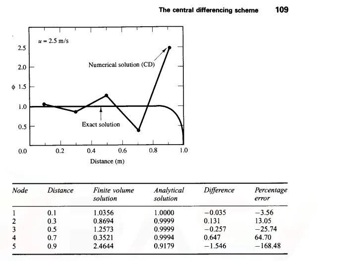The result obtain from the input details for the discretize equation shows that the numerical solution Wiggles around the Exact solution.

This is due to the fact that Central Differencing Scheme calculate the flux from all its neighbouring points and have not recognized the flow direction does not obey Transportiveness.For such cases we develop other interpolation schemes :

• Upwind Differencing Scheme
• Hybrid Differencing Scheme
• Power-Law Scheme
• Quadratic Upwind Differencing Scheme (QUICK)

For the Upwind Differencing Scheme this scheme takes the flow direction into the account and can calculate the cell face value according to it.If the flow direction is positive that will make the phi value as,

`phi_W = phi_w` and `phi_e = phi_P`

• Flux Limiters.

For convective fluid flow, it is observed that the low order schemes are usually stable but quite dissipative in nature around the points of discontinuity or shocks while the higher order schemes are unstable in nature and show oscillations in the vicinity of discontinuity or shocks. Highly accurate and oscillation free schemes are known as High Resolution Schemes.

Flux Limiter functions are used to fine tune the higher order and lower order schemes in such a way that the resulting scheme gives a higher order accuracy in the smooth region of the flow and maintains first order accuracy in the vicinity of shocks and discontinuities. For such a scheme TVD scheme is employed.

`F_(i+1/2) = L_(i+1/2) + phi(H_(i+1/2)-L_(i+1/2))`

where L = 1st order low precission flux

H = highest order high precission flux

`phi` = `(u_(j) - u_(j-1))/(u_(i+1)-u_(i))`