Week 1: Channel flow simulation using CONVERGE CFD
AIM
* To simulate flow through a channel for different mesh size.
* To obtain velocity contour and pressure contour.
* To plot velocity, pressure, mass flow rate, cell count for all the simulated mesh size.
INTRODUCTION
Flow through channels can also be stated as flow through closed pipe, only difference being the cross section of the channel. For flow through pipes the cross section will be circular and for flow through channnels the cross section of the channel will be non-circular, generally a square cross-section or a rectangular cross-section.
Flow through channel can be well explained in terms of its velocity profile and shear stress plot. As fluid flows through the channel, the layers of fluid which is in contact with the channel wall comes to rest and this is called as No-slip condition. Layer which is in conatct with the channel walls trys to pull the layers beneath it, so the layer which is beneath the zero velocity layer slows down or in other words we can say that its velocity decreases. Same apply's for other layers as well. As we move from the walls of the channel to the center of the channel the pull or resistance offered by layers decreases. The layer which is in the centre of the channel will have more velocity compared to its adjacent layers, this criteria gives the velocity across (Radial direction) a parabolic profile.
Haigen poiseuille theory states that the parabolic profile of the velocity is not completley parabollic until the flow is fully developed. From the inlet there is a distance upto which the flow will be developing, this length from the inlet upto which the flow will be developing is called Hydrodynamic entry length `(L_H)` along this distance the parabola is not complete. After the hydrodynamic entry length the flow gets fully developed and hence a complete parabollic velocity profile can be observed. Below is a pictorial representation of the developing parabola.
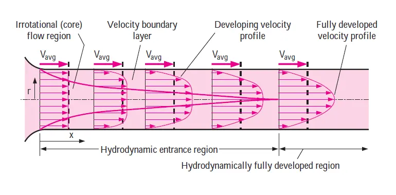
Hydrodynamic entry length for laminar flow is given as `L_H = 0.05 *Re * D`
where `Re -` Reynolds number.
`D -` Characteristic length (m).
Characteristic length varies according to the cross section of the channel. If the cross section is circular then the diameter of the circle equals to the characteristic length. If the cross-section is non-circular then the characteristic length is given as,
`D = (4*A_c)/p`
where, `D -` Characteristic length (m).
`A_c -` Cross-sectional area (m^2).
`p -` Wetted perimeter (m).
For Turbulent flow the hydrodynamic entry length is given as, `L_H = 10*D`
where, `D -` Characteristic length (m).
SIMULATION
* Geometry :
In this simulation a channel with square cross section is used. Dimension of the square cross-section being 0.01 m * 0.01 m, length of the channel is taken as 0.1m. Channel is created in the converge using the create shape option. Channel created for the simulation is as shown below,
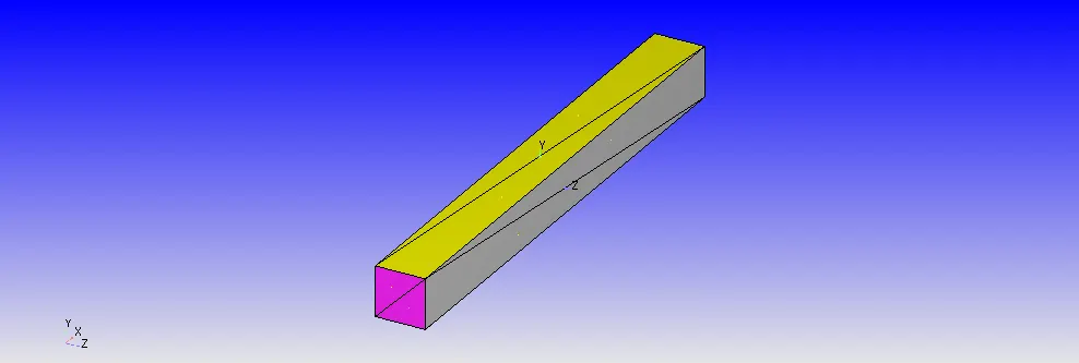
After creating the channel boundary's are flagged, using the boundary options. Inlet, outlet, top-bottom wall, front and back are the names given to the boundary's. While defining the boundary's the front and back are defined such that the normal from the back and front faces are aligned in the z-direction. Below is the snip showing the different boundary with their respective id's.
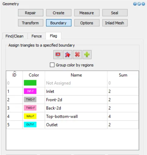
Normal direction should be checked before proceeding further, generally the normal direction should point towards the fluid volume it the normal direction is pointing away from the fluid volume then it can be rectified using the transform option.
* SETUP :
Whole setup which includes initialization, setting up boundary conditions, setting the solver etc. all fall under the case setup window a snip of the casesetup window along with all the parameters set is as shown below,
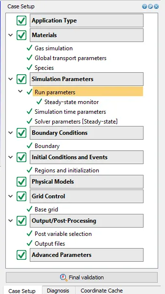
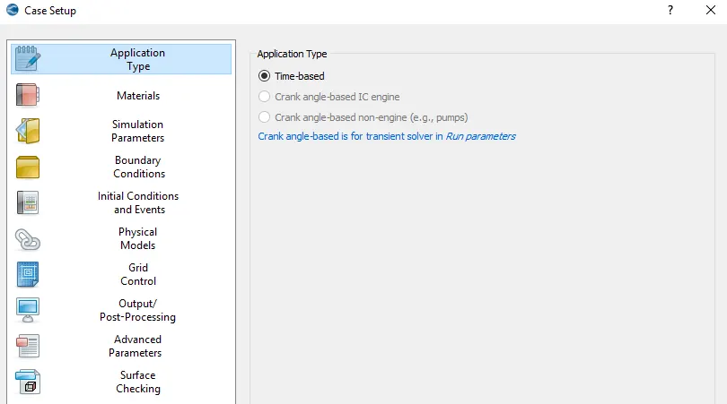
* First we can start from setting the application type as time based, below is the snip of the same.
* After setting up the application type next comes the material type that we can select, on clicking the materials tab a window opens under which there are certain controls related to material properties, a snip of the window is shown below.
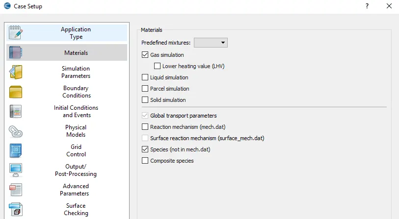
In this the Reaction mechanism is unchecked and species is checked. Once this is done we can set the gas simulation and global transport parameters. For this simulation all the controls under the gas simulation and global transport parameters are left as default. Only thing that is set under the materials tab is Species. A snip of the species parameters set are shown below,
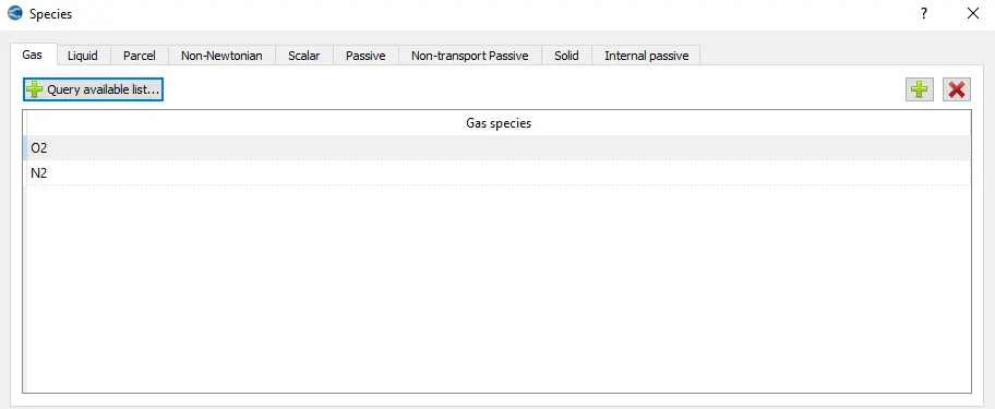
O2 and N2 are the species defined or else it can be stated that air which is the fluid under consideration is composed of O2 and N2.
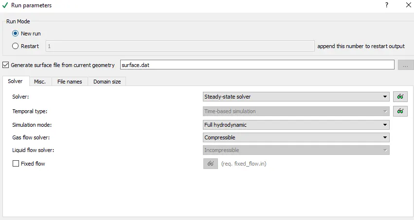
* Once the material parameters are set then we can proceed to set the Simulation parameters. Under this first comes the Run parameters. Below is the snip of the Run parameters in this we are setting the steady state solver also the simulation mode is set to Full hydrodynamic also the gas flow is set as compressible.
* Under the misc tab we can find the controls as shown below,
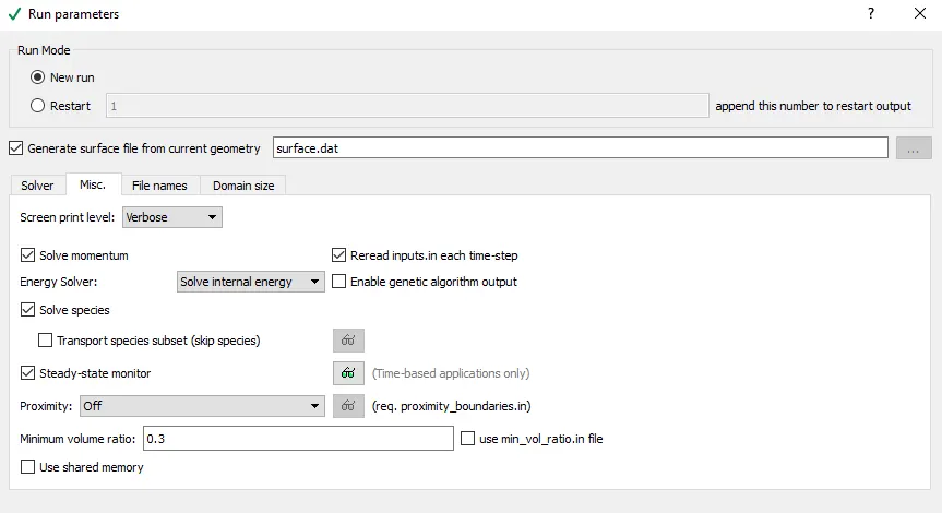
In this the steady state monitor is checked and use shared memory is unchecked. The controls which is under the file name tab and the domain size tab is left as default setting.
* After the Run parameters then comes the steady state monitor,
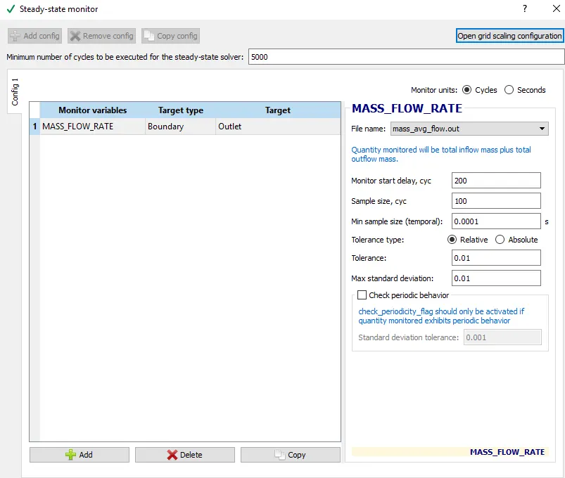
In this mass flow rate at outlet is set as the parameter, Minimum number of cycles to be executed by the steady state solver is set as 5000. Apart from this the Mointor start delay cyc is set as 200 and Sample size cyc is set as 100.
* All the time or cycle related controls can be seen in simulation time parameters tab.
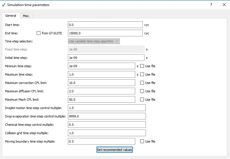
In this end start time is set as zero and end time is set as 15000 cyc. Initial time step, minimum time step is set as 1e-9 and maximum time step is set as 1.Apart from this all other controls are left as it is.
* After simulation time parameters there comes solver parameters.
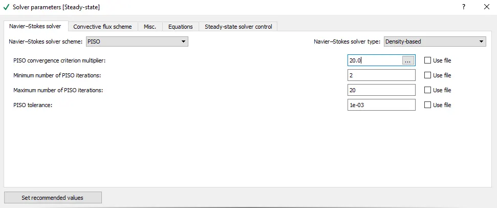
Under the Navier-stokes solver parameters solver type is set as density type. Under the misc tab the strict conserve control is set as 0-No strict conserve. 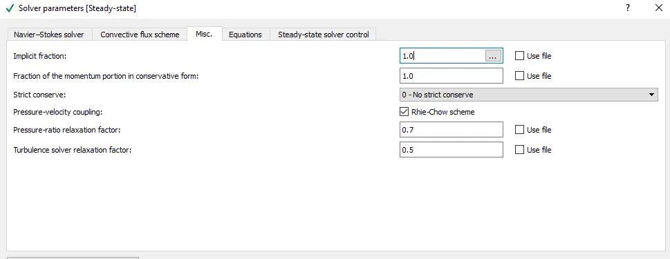
Below is the snip of Equations tab,
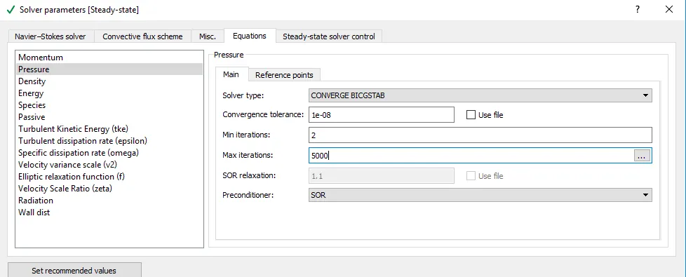
Under this the Max iteration for pressure is set as 5000. This is set after running the simulation for the first time wherein the simulation stopped at 25th iteration showing a warning that the "Max iteration for pstar is exceeded" hence the max iteration for pressure is set as 5000. Apart from pressure all other parameters under the Equations tab is left as it is.
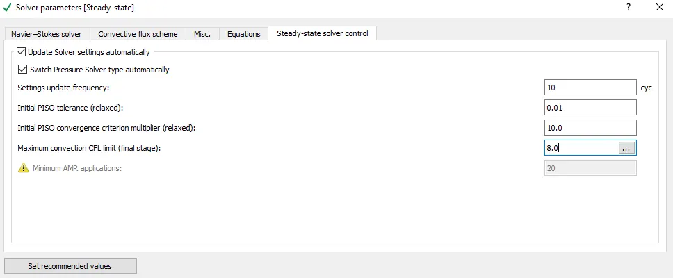
* Under steady state solver control tab update solver settings automatically and switch pressure solver type automatically is checked. Maximum convection CFL limit (Final stage) is given a number less than the value given to Maximum convection CFL limit set undre the smulation time parameters. A snip of the same is provided below,
* Once all the simulations parameters is set then comes the Boundary conditions:
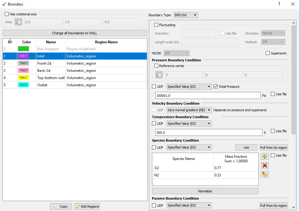
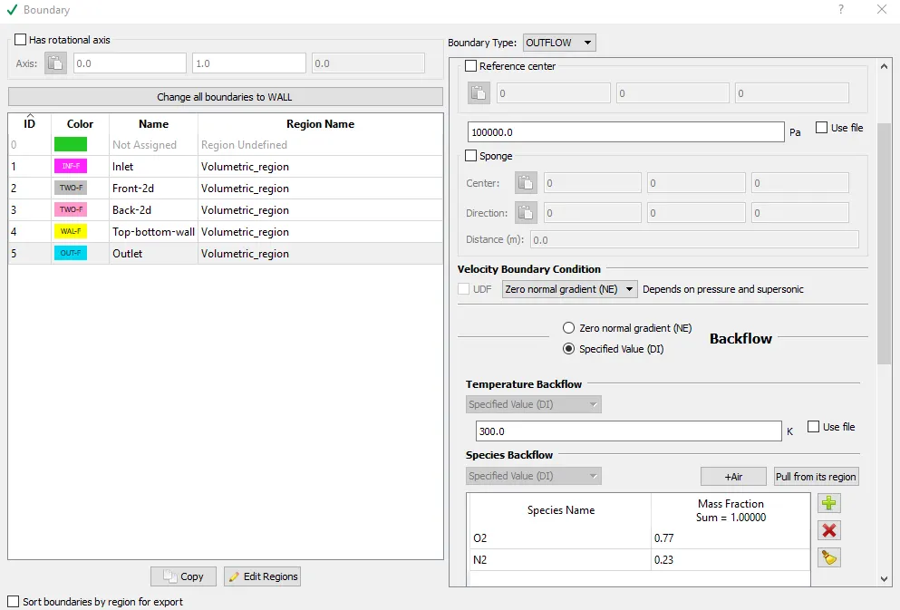
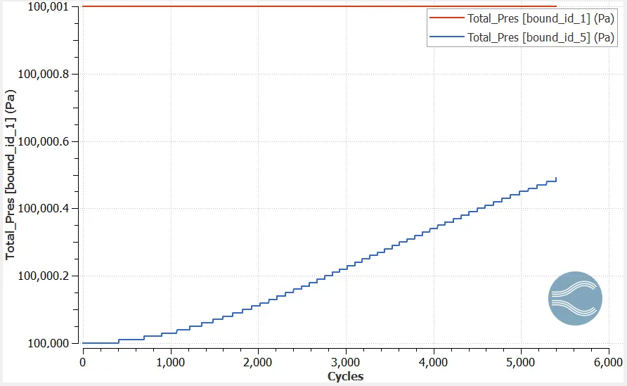
1. Inlet: For inlet inflow B.C is set. pressure at the inlet is specified as 100001 Pa also inlet temperature is set as 300 K. Also the fluid under consideration along with the species needs to be specified here including the mass fraction of the species. Mass fraction of O2 is set as 0.77 and that of N2 is set as 0.23.
2. Outlet: Outflow B.C is set also the outlet pressure is set as 100000 Pa and temperature is set as 300 K. Same as inlet the fluid along with its species and respective mass fraction need to be specified.
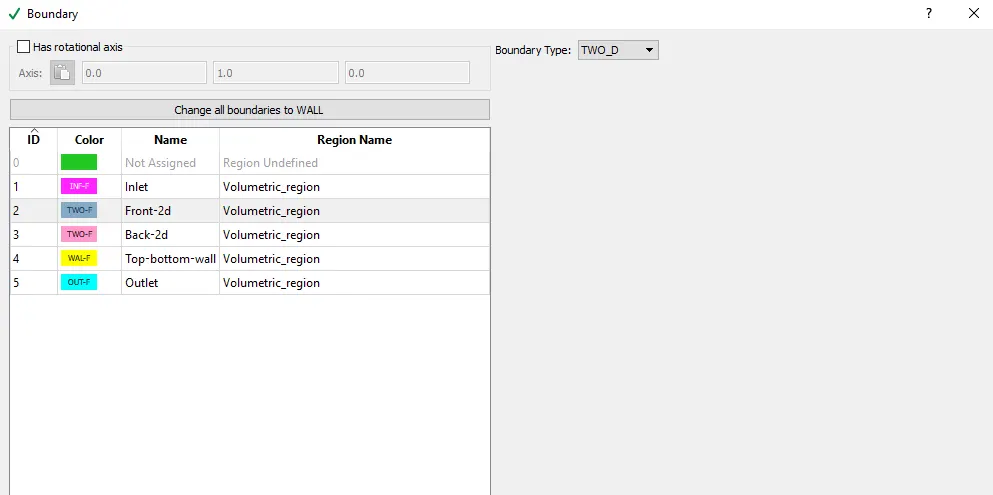
3. Front and Back faces: 2-D B.C is set for these 2 faces.
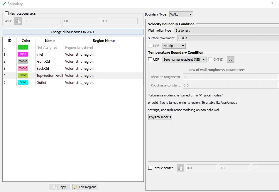
4. Top-Bottom wall: For this wall is the B.C set. Under this the wall motion type is set as stationary also the surface movement is set as fixed with No-slip condition.
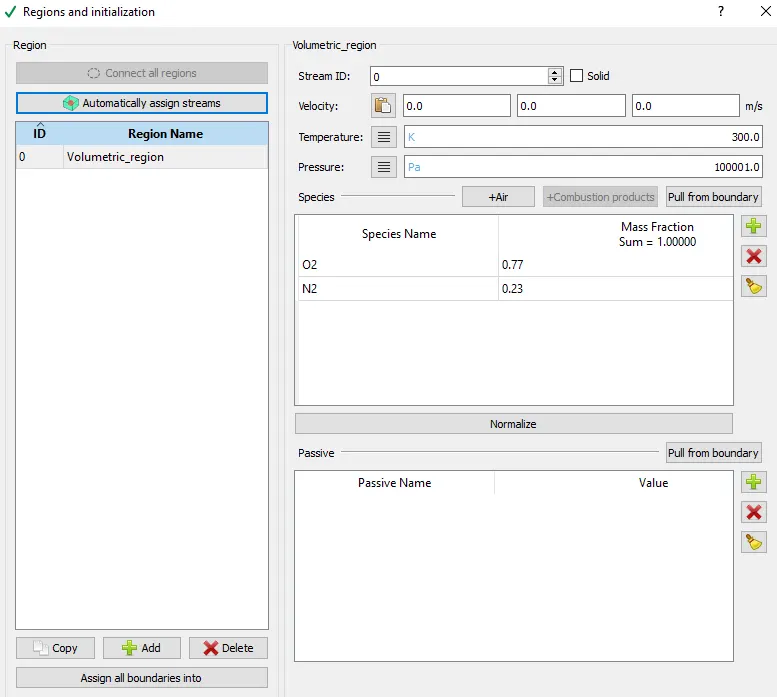
* After setting up the Boundary condition we can initialise the solution. This can be done using the controls under the Region and initialization option. Where we can set a name for the region also the initial pressure at is set same as inlet pressure. Species along with its mass fraction needs to be mentioned here.
* Grid size is very improtant characteristic of a simulation this parameter can be set using the Grid controls.
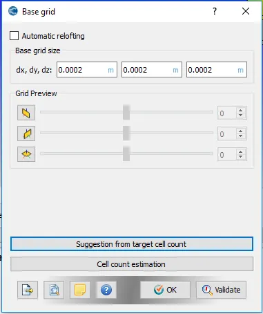
In this simulation is being carried for 3 different mesh sizes.
* Output file contorls can be seen under output/post processing tab. In here the time interval for writing 3D data output files is set as 100 cyc and Time interval for writing restarting output is set as 1000 cyc.
Setting up the all the above mentioned parameters completes the case set up for this simulation. Next step is to run the simuation this can be done using the cygwin command prompt. Before proceeding with the running the simulation it is must that we first export the input files (which includes all the parameters set above) into a directory. This can be done using the export option present under the file. Once export of files are done the next thing is to copy 2 files namely converge-intelmpi.exe and mpiexec.exe from the converge directory to the directory where the input files are exported. After this using the cygwin comand prompt we should navigate to the directory where the input files are exported and then " mpiexec.exe -n 4 converge-intelmpi.exe restricted" command is typed to run the simulation.
As stated before this simulation is carried out for same B.C for 3 different mesh sizes. Results of the simulations is disscussed below.
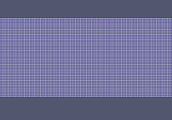
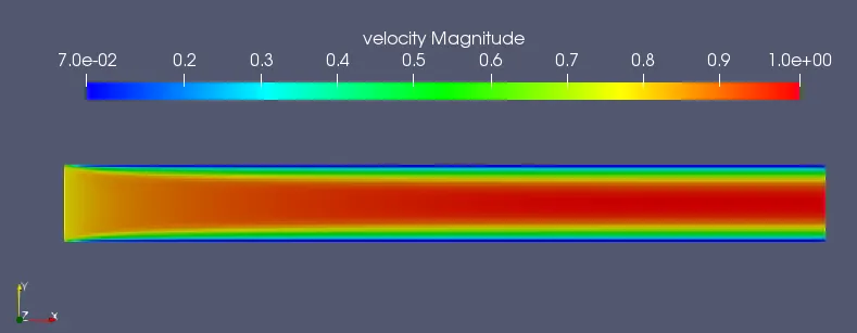
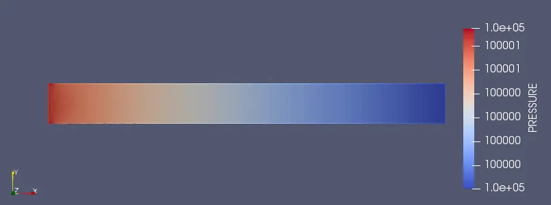
1. Mesh size = 2e-4.
* Meshed surface:
* Velocity contour:
* Pressure contour:
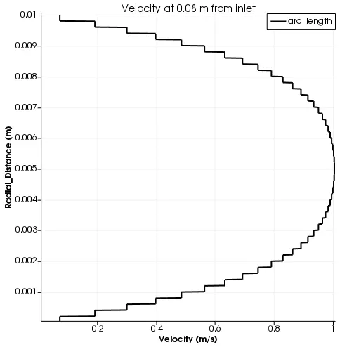
* Velocity profile at outlet:
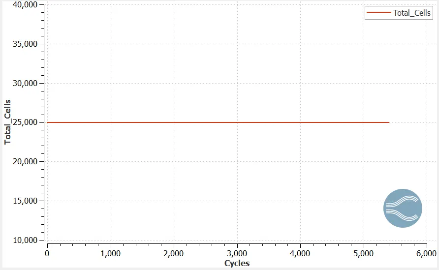
* Mesh count plot:
* Total pressure plot of inlet and outlet:
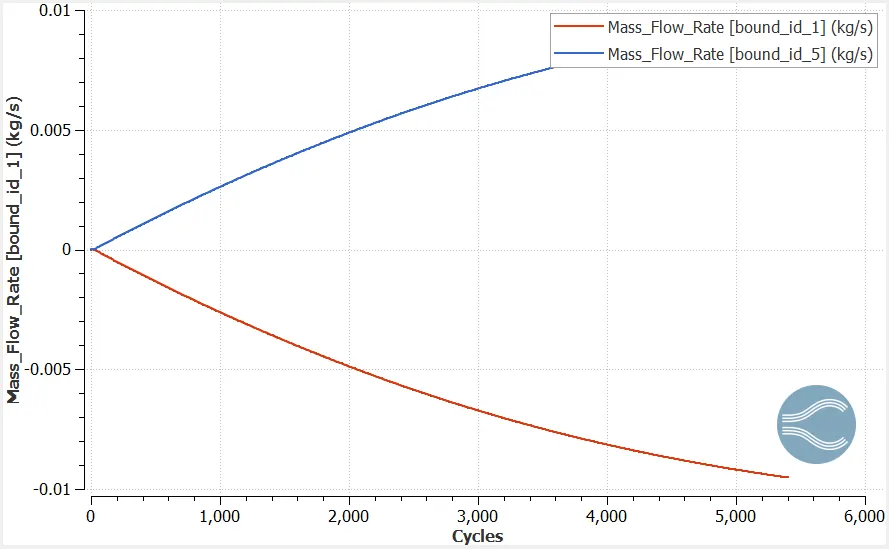
* Plot of mass flow rate at inlet and outlet:
Velocity_contour_animation - https://youtu.be/CArKgC3CGH4
2. Mesh size = 1.5e-4.
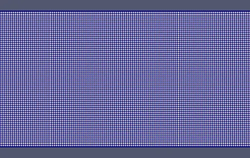
* Meshed surface:
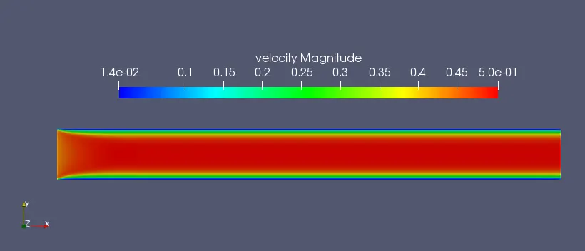
* Velocity contour:
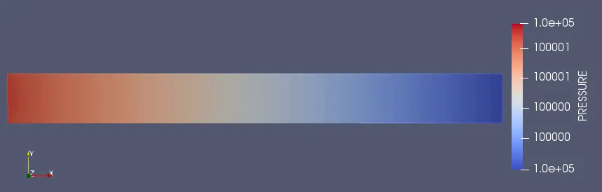
* Pressure contour:
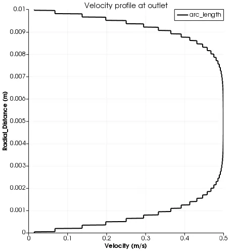
* Velocity profile at outlet:
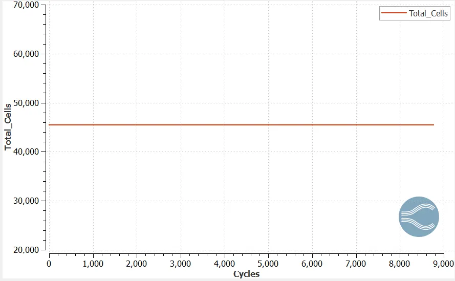
* Mesh count plot:
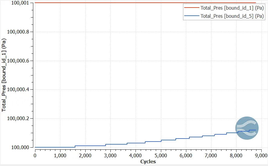
* Total pressure plot of inlet and outlet:
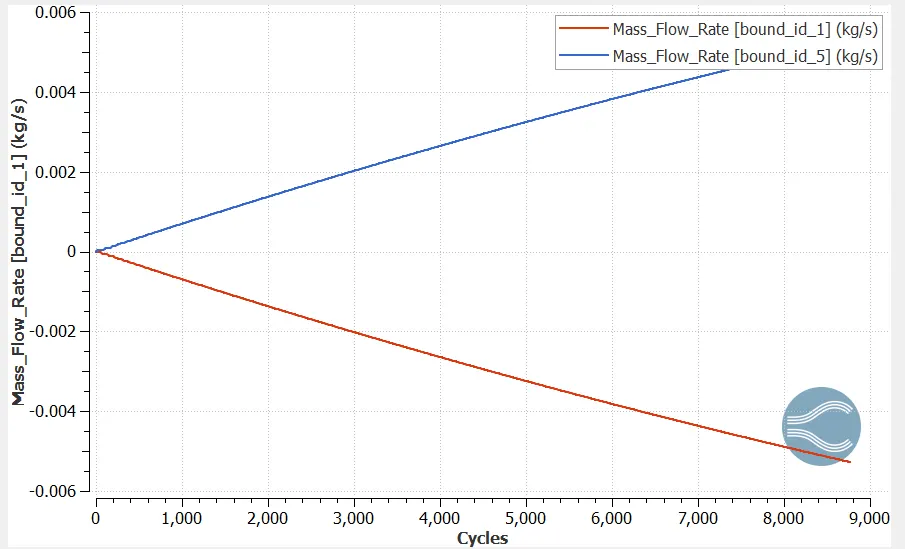
* Plot of mass flow rate at inlet and outlet:
Velocity_contour_animation - https://youtu.be/sDCD7Eq-MFE
3. Mesh size = 1e-4.
* Meshed surface:

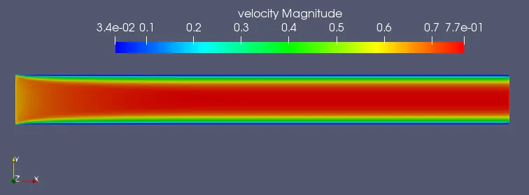
* Velocity contour:
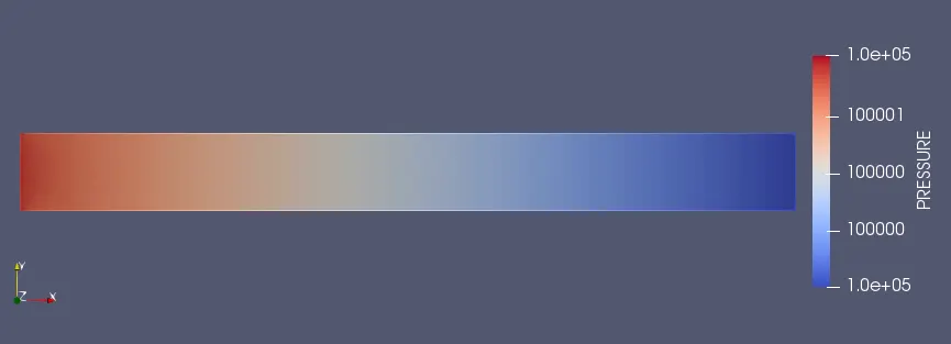
* Pressure contour:
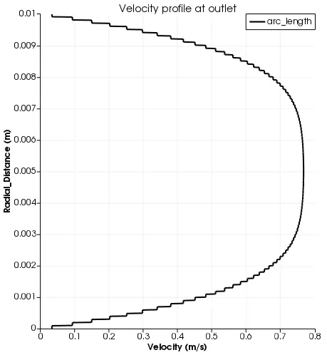
* Velocity profile at outlet:
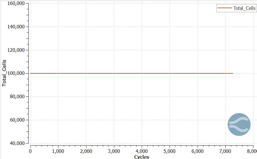
* Mesh count plot:
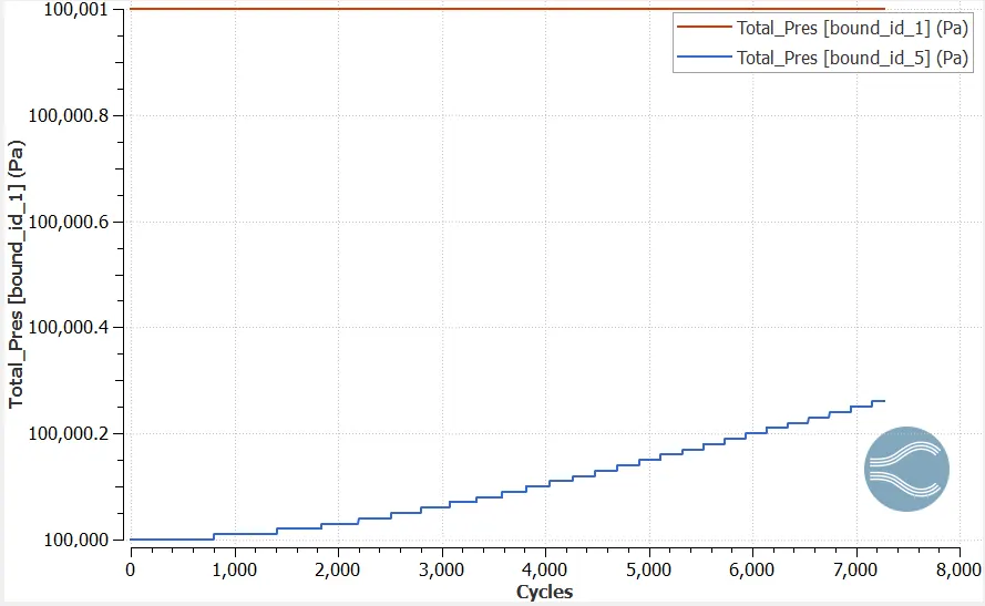
* Total pressure plot of inlet and outlet:
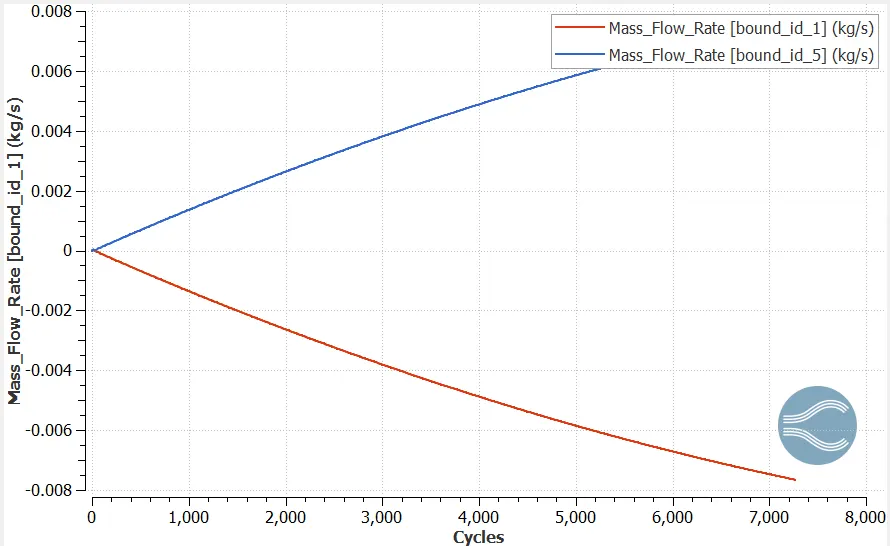
* Plot of mass flow rate at inlet and outlet:
Velocity_contour_animation - https://youtu.be/PUNmGfkJ2HQ
* As per Haigen poiseuille theory as disscussed above until the hydrodynamic entry length the flow is developing accordingly the parabollic velocity profiles will be developing. Since inlet pressure and outlet pressure were set as boundary condition so before starting the simulation we cannot compute the Re. After completing the simulation using post processing tool paraview we can take a plot overline at inlet and from the plot obtained we can calculate the inlet velocity.
so first case of mesh size = 2e-4 is considered, from plotoverline the inlet velocity is calculated as V = 0.42 m/s.
we have `R_e = (U*D)/nu`
`U` = 0.42 m/s
`D` = 0.01 m (for non circular cross section D =(4*A)/p, i.e D =(4*0.01*0.01)/(4*0.01) = 0.01 m)
`nu` = 1.5757e-5 m^2/s. (Kinematic viscosity of air at 300 K).
Therefore, `R_e = (0.01*0.42)/(1.5757e-5) = 266.5`
Hydrodynamic entry length for laminar flow is given as `L_H = 0.05*R_e * D`
therefore, `L_H = 0.05 *266.5*0.01 = 0.133 m` i.e Till this length the flow will be developing and hence only after this length we can obtain a complete parabollic velocity profile. Since in this simulation the length of the geometry is fixed to 0.1 m, a completley developed flow can't be observed.
For other 2 cases also it is observed that the fully developed flow is obtained for a hydrodynamic entry length more than 0.1 m.
CONCLUSION
1. For different mesh sizes the max velocity obtained at the outlet must be almost equal but by observing the velocity contour's of all 3 cases it is clear that the max velocity at the outlet vary's considerably which implies that the soution is not converged. Same can be validated by observing the mass_flow_rate plots, where it can be seen that mass_flow_rate is varying with the number of cycles.
2. As the size of mesh is decreased the cell count increased also the time taken for the simulation to run is also increased.
3. Since the total length of the channel is fixed at 0.1 m a fully developed flow cannot be observed.