Week 4: Project - Steady state simulation of flow over a throttle body
AIM
* To run a steady state simulation of flow through a throttle body.
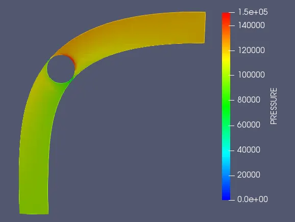
* To show the meshed surface, velocity and pressure contour.
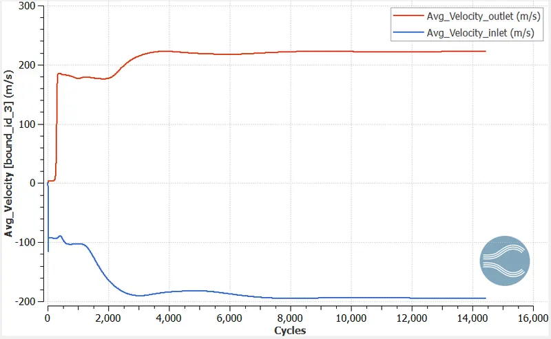
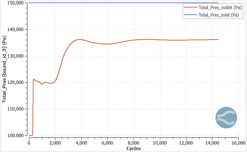
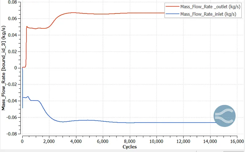
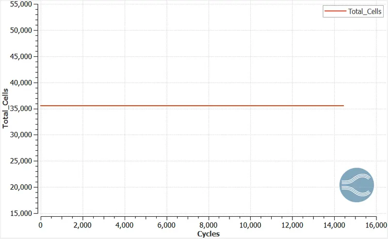
* To show plots for velocity, pressure, mass flow rate, total cell count.
INTRODUCTION
Steady state simulation of flow through a throttle body can be related to flow through a pipe, only difference being the presence of a throttle body. It is very much intutive that throttle is used to control the flow through the pipe but rotation of throttle being a time dependent process it cannot be included in steady state analysis and hence in this simulation throttle will be stationary. Fluid will flow past the throttle, since there is no rotation of the throttle there wont be any controlling of the flow.
SIMULATIONS
Geometry:
The throttle body used for this simulation is a 'L' shaped elbow like structure inside of which is the throttle body which is intended to control the flow. Below is the snip of the geometry
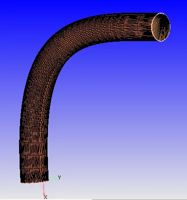
hiding some of the surface triangles makes the throttle visible. A snip of the same is provided below,
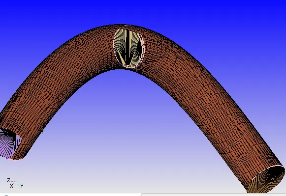
In practice the throttle will be mounted on a rotating axis, both ends of the rotating axis will be attached to the throttle wall. In this case the rotation axis is not attached to the throttle wall so that some intersection error can be avoided.
Case setup:
* Geometry is first opened in the converge, after that a diagnosis is run to check wether there are any surface errors. Below is the snip of the same.
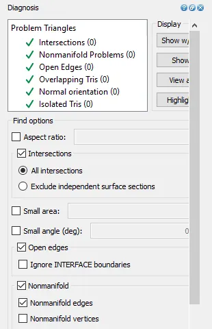
* From the above output it is clear that there are no surface errors and hence we can proceed further in setting up the simulation.
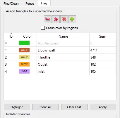
* First Boundary's are flagged, below is snip of the boundary's flagged along with the boundary id.
* Gas is selected as the fluid and accordingly gas simulation is checked while setting up the case. Along with it the reaction mechanism is unchecked and species is set.
* Under materials tab gas simulation and global transport properties are set default. Under species local control `N_2, O_2`are the species set. Snip of the same is provided below,
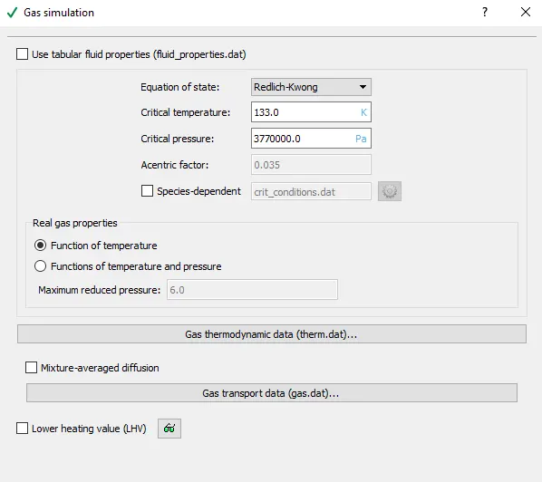
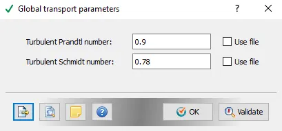
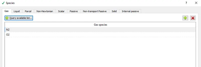
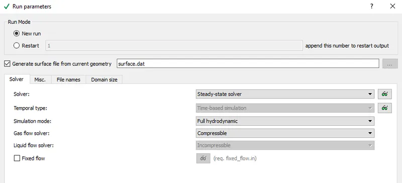
* Under run parameters a steady state solver is set, to run a full hydrodynamic simulation. Gas flow solver is set to compressible.
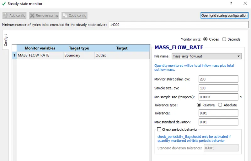
* Under steady state monitor minimum number of cycles to be executed is set at 14000 cycles, mass flow rate at outlet is set as monitor variable along with other local controls. Snip of the same is provided below,
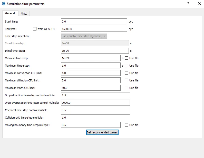
* Under simulation time parameters start time and end time are set at 0 and 15000 cycles respectivley. Also initial time step and minimum time step is set to 1e-9 along with max time step set at 1.
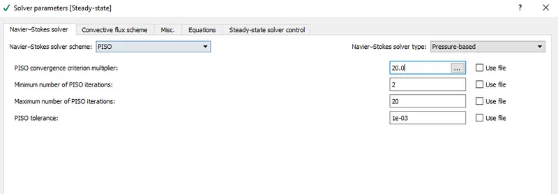
* A pressure based solver is set.
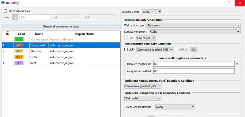
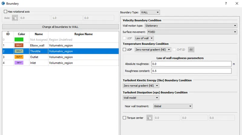
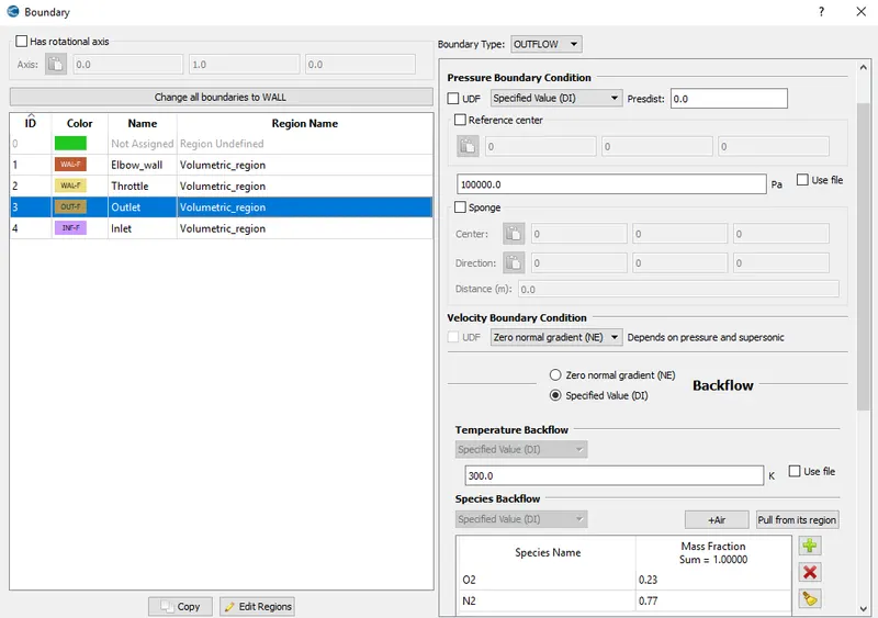
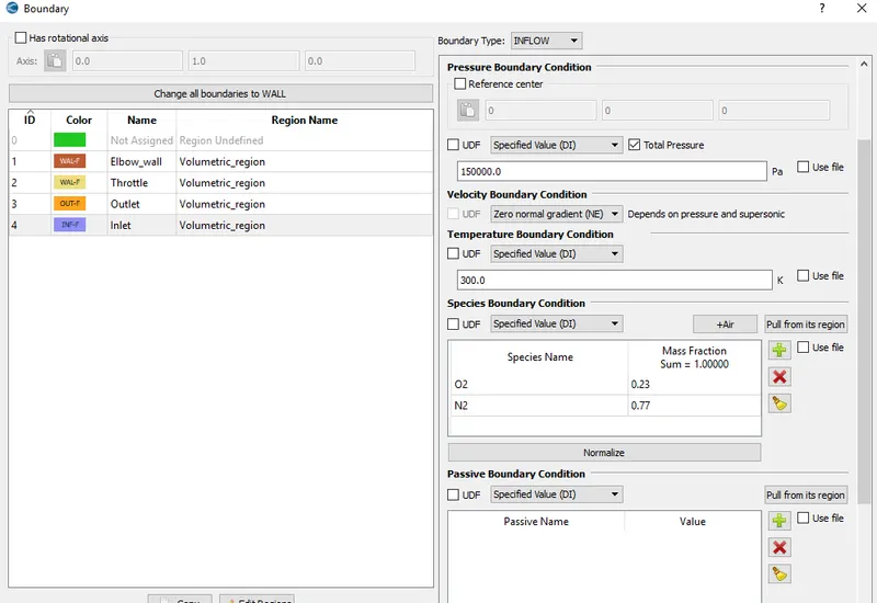
* Next is setting up the boundary conditions. For elbow_wall and throttle boundary type is set as wall. Wall motion type is set as stationary and surface movement is set fixed. For inlet boundary type is defined as inflow with a inlet pressure of 150000 Pa and a temperature of 300 K, also inlet species `O_2 , N_2` are defined along with their mass fractions. For outlet boundary boundary type is set as outflow with outlet pressure of 100000 Pa and inlet temperature of 300 K here also the species `O_2, N_2`are defined. Snip of above mentioned 4 boundary conditions is given below,
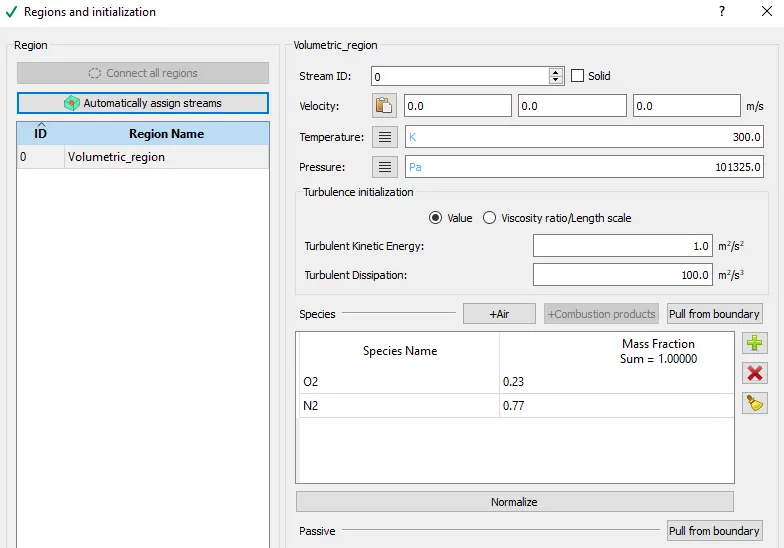
* Fluid volume is initialised by setting up regions and initialization local control. Temperature of 300 K and pressure of 101325 Pa is set and the region is flagged as Volumetric_region.
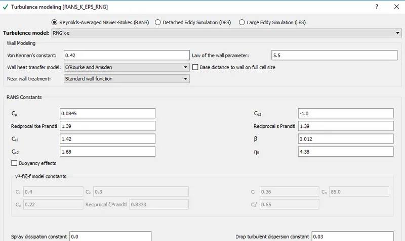
* Under physical models RNG K-ε turbulence model is selected.
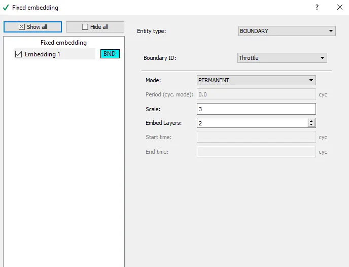
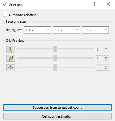
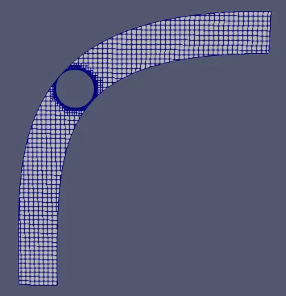
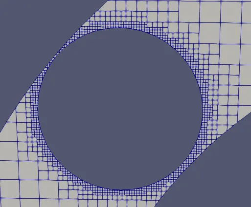
* A grid of 0.002 m is set in all 3 directions along with that fixed embedding is provided to the throttle boundary. A embedd scale of 3 and number of embedd layers 2 is set.
* Simulation is run with above mentioned case setup and results are noted. Results are disscussed below.
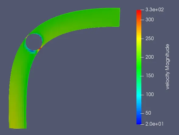
* Velocity contour:
* Pressure contour:
* Velocity plot:
* Pressure plot:
* Mass flow plot:
* Cell count plot:
* Meshed surface:
* Embedd layers:
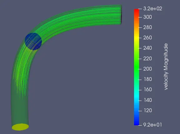
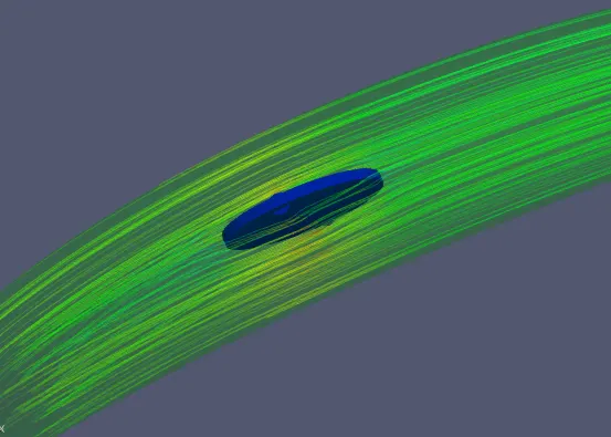
* Velocity Streamlines:
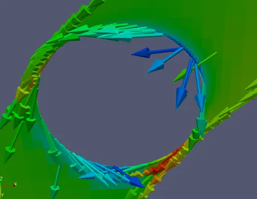
* Glyph:
* Velocity profile animation:
Observation:
* Since the throttle valve is not rotating near the throttle valve flow is not chaotic.
* When the fluid gets hit to the throttle valve there is be sharp decrease in velocity, this is clearly visible while observing the velocity contour plot.
* Since there is a velocity decrease at the throttle there is a recirculating region around the throttle this can be verified by observing the glyph plot.