Week 10: Project 1 - FULL HYDRO case set up (PFI)
AIM
* To run full hydro simulation on a PFI engine.
* To generate different plots such as integrated heat release rate, volume, pressure, spary distribution etc.
* To calculate compression ratio of the engine from volume plot.
* To calculate combustion efficiency of the engine using the integrated heat release plot.
* To calculate work done, torque from the engine using the engine performance calculator of the converge.
* To briefly explain significance of ca10, ca50, ca90.
* To briefly explain the significance of using a wall heat transfer model.
INTRODUCTION
PFI engine refers to port fuel injected engine's. A model PFI engine is used to run the simulation, since combustion simulation is a time taking process, before running a full fledged (full hydro) simulation a no hydro simulation is run, to check how the mesh generation takes place and how the valve movements are. No hydro simulation is started by flagging the boundary's and then surface preparing the geometry. Detailed explaination of the no hydro simulation is explained in the previous challenge.
In full hydro simulation apart from the case setup disscussed in the no hydro simulation there are other things such as setting up of spray model, combustion model, embedding's etc. which will be disscussed. In full hydro simulation the Navier stokes equation along with species transport equation will be solved and hence completing the combustion simulation.
SIMULATIONS
Geometry:
The PFI engine geometry used for the simulation is as shown below
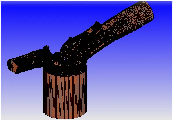
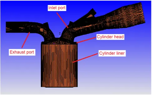
Above gemoetry is checked for surface errors and the suface errors are corrected before setting up the case.
Case setup:
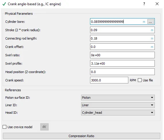
* Case setup is started by setting the application type as crank angle based - IC engine. Under this setting need to set the bore, stroke, connecting rod length, crank offset, crank speed etc.
* Above mentioned parameters are set, a snip of the same is given below,
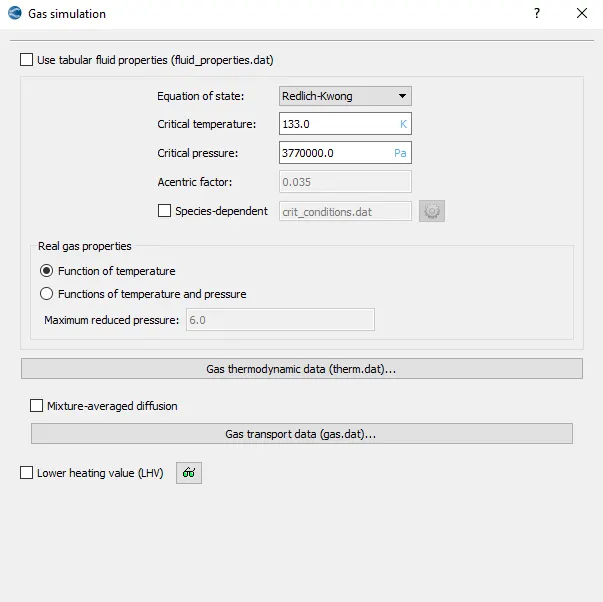
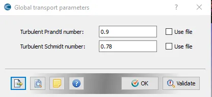
* Gas simulation is used to run the simulation, under this local control real gas properties is set as function of temperature and gas thermodynamic data is imported. Since gas phase simulation is selected importing thermo dat file imports thermodynamic data of all gas species concerned with the combustion reaction. Global transport properties are set default.
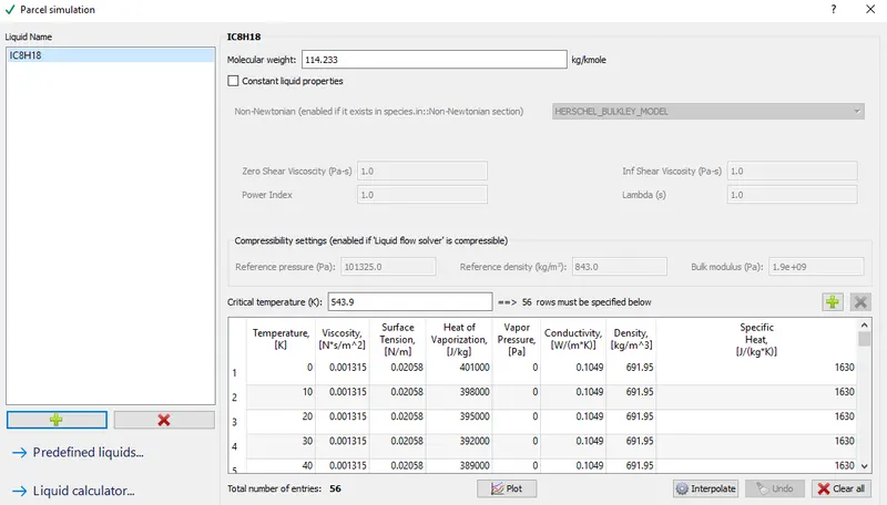
* Since this is full hydro simulation parcel simulation option is selected, so under materials it is necessary to set the parcel. In this simulation iso-octane (`iC_8H_18`) is the fuel used and hence it is set as the parcel.
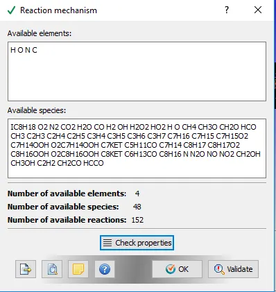
* Since this is a combustion reaction, reaction mechanism needs to be specified, hence the mech.dat file which consists of reaction mechanism concerned with gasoline is imported.
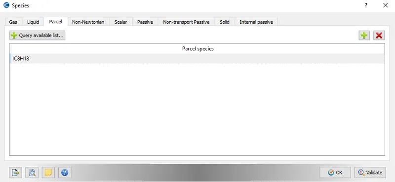
* Under species local control it is set as type parcel and `iC_8H_18` is set as the parcel.
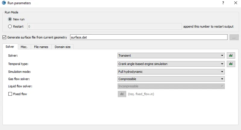
* Next Simulation parameters are set under which first comes the run parameters. A transient , full hyrodynamic simulation is set. Gas flow solver is set as compressible. All other local controls under run parameters are set to default values.
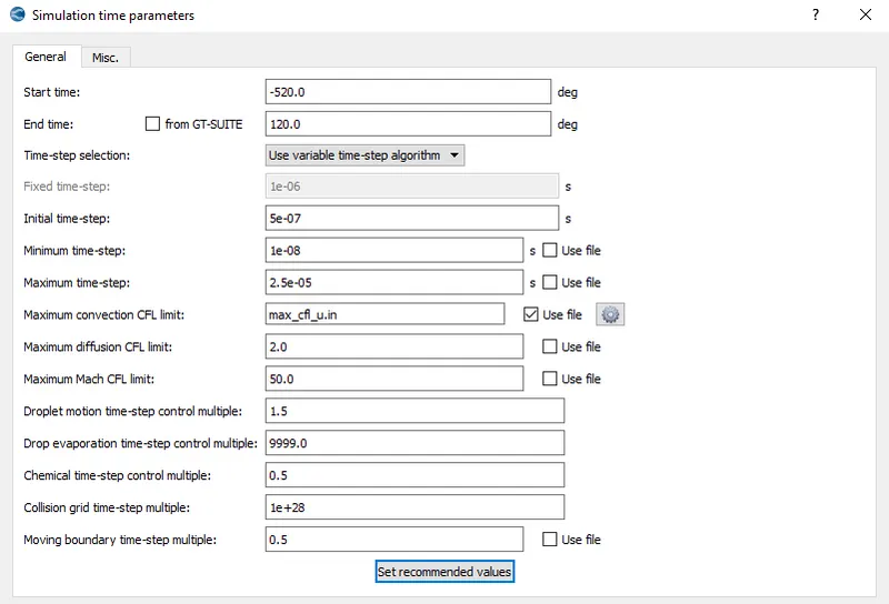
* Second comes the simulation time parameters, since this is crank angle based simulation the start time and end time needs to be set in degree's. Start time of -520 deg and end time of 120 deg is set along with a initial time step value of 5e-07 sec and min time step of 1e-08. Other local controls are specified as shown in below snip,
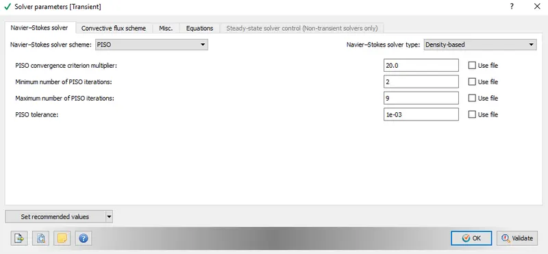
* Under solver parameters a density based solver is set and all other local controls are set to default values.
* Before setting up the boundary condition it is necessary to set the regions.
* Total of 4 regions were defined which are as follows:
1. Cylinder_region - Temperature of 1360 K is defined along with pressure of 185731 Pa. Species that belong to the cylinder region needs to be defined along with its mass fraction, to do that we need to consider the following stoichometric reaction,
C8H18+12.5⋅(O2+3.76⋅N2)=8⋅CO2+9⋅H2O+(3.76⋅12.5)⋅N2">C8H18+12.5⋅(O2+3.76⋅N2)=8⋅CO2+9⋅H2O+(3.76⋅12.5)⋅N2C8H18+12.5⋅(O2+3.76⋅N2)=8⋅CO2+9⋅H2O+(3.76⋅12.5)⋅N2
so the product species of the above stoichometric reaction is defined as species for the Cylinder_region. Mass fraction of product speices are calculated as shown below,
| Species | Number of moles | Molecular weight | Mass fraction |
| `CO_2` | 8 | 44.01 | 0.192 |
| `H_2O` | 9 | 18.015 | 0.088 |
| `N_2` | 47 | 28.0134 | 0.7191 |
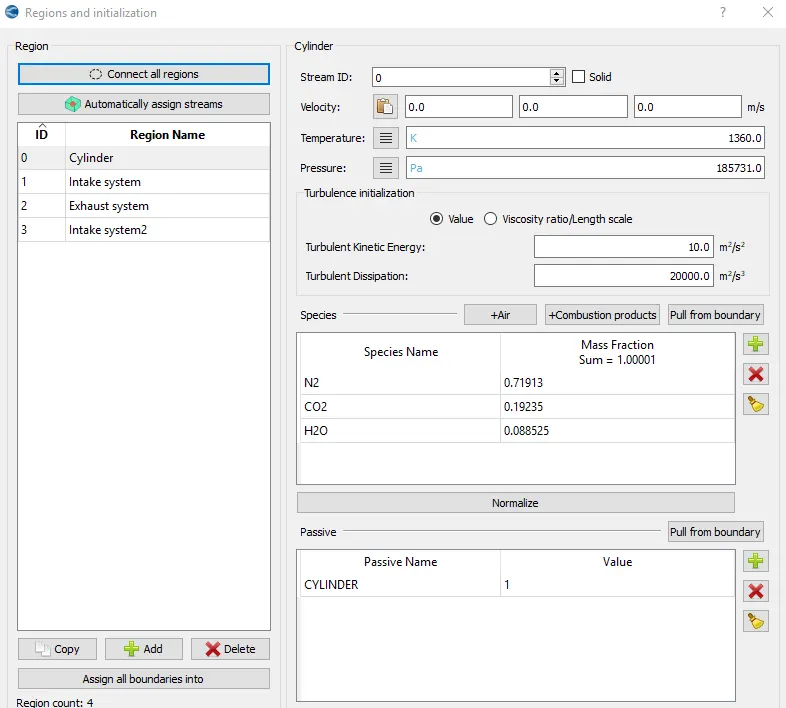
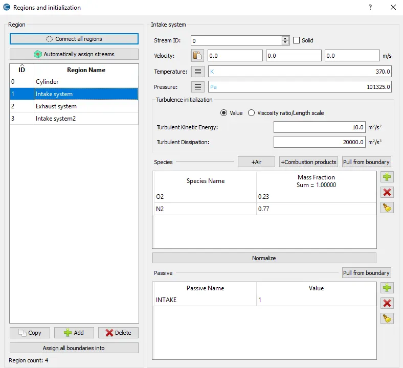
2. Intake system - Temperature of 370 K and a pressure of 101325 Pa is defined in this region, this region is one half of the intake port which interacts with Intake system2. Species which belong to this region are C2H18,O2andN2">O2 and N2 mass fraction of these species are set.
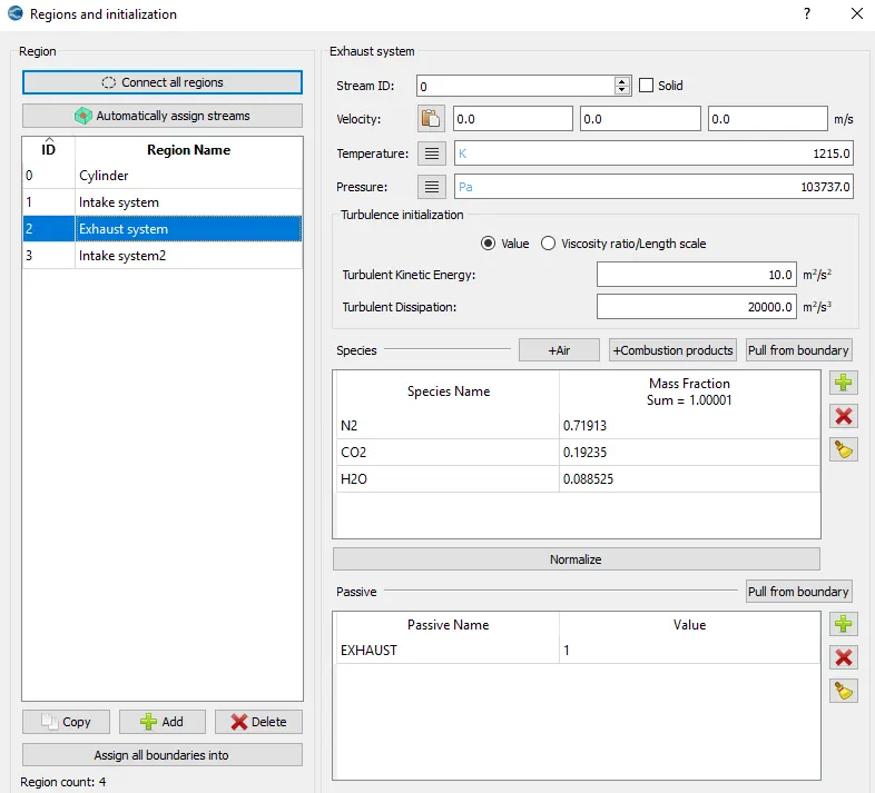
3. Exhaust system - This region interacts directly with cylinder region and hence same species defined for the cylinder region is defined for this region as well. Temperature of 1215 K and a pressure of 103737 Pa is defined for this region.
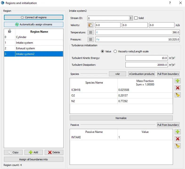
4. Intake system2 - this region is the another half of the intake port which interacts with cylinder region. Temperature of 390 K and pressure of 101325 Pa is defined. Species which belong to this region are `iC_8H_18, N_2, O_2` mass fraction of these reactant species is calculated in same way as shown above.
* Once regions are defined and initialised B.C are defined for each boundary. Details of the boundary condition applied is shown below,
* Piston : Boundary type - Wall
Wall motion type - translating
Surface movement - Moving, piston motion.
Temperature = 450 K
* Liner : Boundary type - Wall
Wall motion type - Stationary
Surface movement - Fixed
Temperature = 450 K
* Inflow : Boundary type - Inflow
Pressure =101325 Pa
Temperature = 363 K
Species defined - `N_2, O_2`
* Outflow : Boundary type - outflow
Pressure = 101325 Pa
Temperature = 800 K
Species defined are `N_2, O_2, H_2O`along with the mass fractions which are calculated in the above shown table.
* Cylinder head : Boundary type - Wall
Wall motion type - stationary
Surface movement - Fixed
Temperature = 450 K
* Exhaut port : Boundary type - wall
Wall motion type - stationary
Surface movement - fixed
Temperature = 500 K
* Exhaust valve top : Boundary type - wall
Wall motion type - translating
Surface movement - moving
Temperature = 525 K
* Exhaust valve angle : Boundary type - wall
Wall motion type - translating
Surface movement - moving
Temperature = 525 K
* Exhaust valve bottom : Boundary type - wall
Wall motion type - translating
Surface movement - moving
Temperature = 525 K
* Intake port : Boundary type - wall
Wall motion type - stationary
Surface movement - fixed
Temperature = 425 K
* Intake valve bottom : Boundary type - wall
Wall motion type - translating
Surface movement - moving
Temperature = 480 K
* Intake valve angle : Boundary type - wall
Wall motion type - translating
Surface movement - moving
Temperature = 480 K
* Intake valve top : Boundary type - wall
Wall motion type - translating
Surface movement - moving
Temperature = 480 K
* Spark plug : Boundary type - wall
Wall motion type - stationary
Surface movement - fixed
Temperature = 550 K
* Spark plug terminal : Boundary type - wall
Wall motion type - stationary
Surface movement - fixed
Temperature = 600 K
* Intake port 2 : Boundary type - wall
Wall motion type - stationary
Surface movement - fixed
Temperature = 425 K
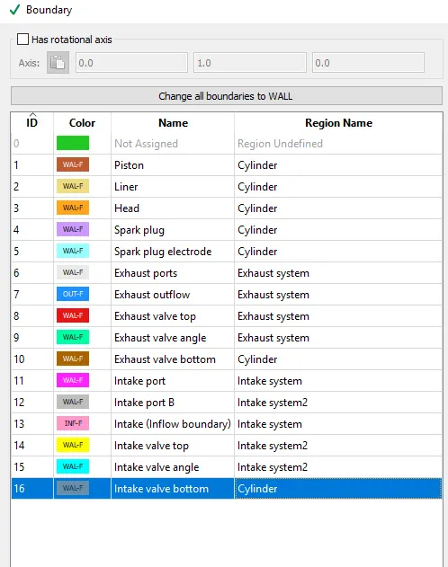
A snip of all the Boundary's along with the regions assigned to each boundary is shown below,
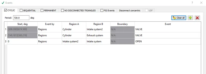
* Next important thing is creating events, which defines when does the regions shall interact. In here events are created between intake system2 and cylinder region, exhaust system and cylinder region and finally between intake system and intake system2. In the above defined events intake system and intake system2 should always interact, there should not form any disconnect triangles and hence they are set open whereas the other two events are controlled using the valve. Below is the snip of the same,
* Setting up the physical model is very much important in this simulation. We can start with spray modelling, before further discussing setting up the spray model local controls it will be better to understand little bit about how spray is modelled.
In converge spray is said to be composed of lagrangian parcels or simply parcels, parcels are spherical shaped each parcel is composed of several drops. So modelling spray means modelling a mathematical equation so that physics related to the spray is well captured. When a parcel traverse through air there will be drag because of which the parcel splits to small parcels called as primary breakup. Parcels which are formed as a result of primary breakup further breaks up this is called secondary breakup. The parcels formed after the secondary breakup starts evaporating because of which there will be decrease in radius of the drop. So as to capture all these physical process concerned with the parcel a good spray modelleing is necessary and converge provides the same.
* We can start with specifying the parcel distribution in inside the spray cone. There are two approaches one in which the parcels are clustered at the centre of the cone axis, second one in which the parcels are evenly distributed within the spray cone. For this simulation even distribution is set.
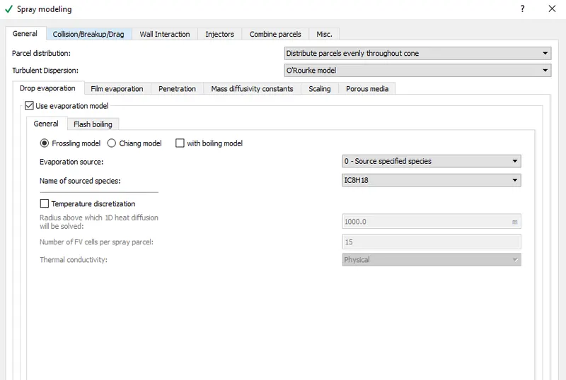
* As explained above as parcel evaporates the radius of the parcels decreases, also after evaporation there will be increase in mass of eulerian gas phase this is compensated by adding the source term in species transport equation. To capture the evaporation and concerned physical aspects converge provides 3 models namley chiang model, frossling model and boiling model. For this simulation frossling model is selected and source specified species is selected.
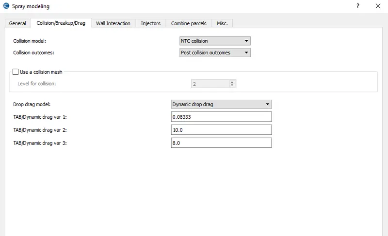
* As far collision models are concerned converge provides two collision models they are NTC collision model and O rourke model, in this simulation NTC collision model is used.
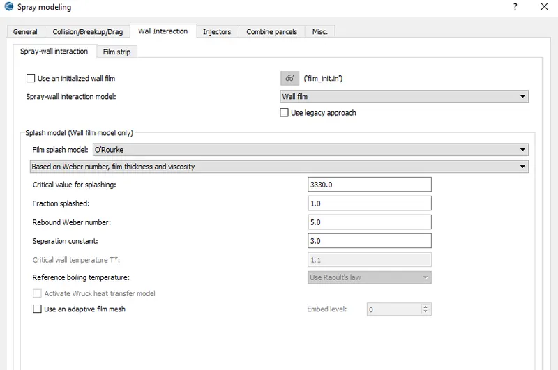
* As far as wall interaction of spray is concerned converge provides 3 models. Spray parcels after hitting the wall, it may rebound, it may form a film on the wall or it may vanish. So for this simulation wall interaction is set as wall film. Other local controls are set as default values.
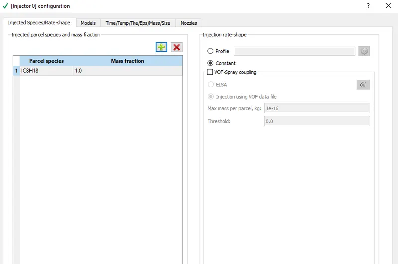
* One of the important local control under the spray modelling is injectors. First is injected species/rate shape, in here the parcel species is set and injection rate shape profile is set.
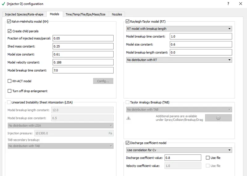
* Next comes model selection for spray, converge provides 4 models namley Kelvin-helmholtz model (KH), Rayleigh taylor model (RT), linearized instability sheet atomization model (LISA), Taylor analogy breakup (TAB) model. For this simulation KH and RT models are selected, there are several local controls available under these two models values for each of those controls can be set using 'set recommendations for' option. Under this option gasoline is selected. Under discharge coefficient model discharge coefficient value is set to 0.8.
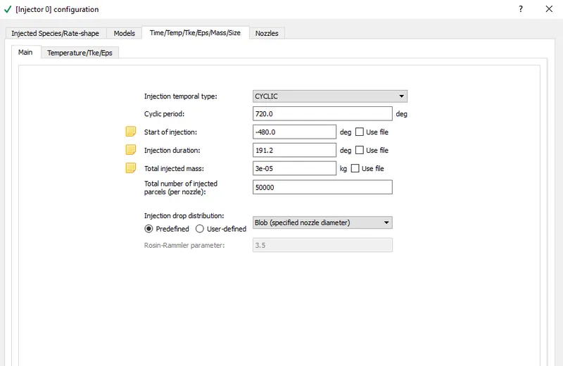
* Next is setting up time/tke/temp/eps/mass size, in here the injection start time and duartion of injection is set in terms of crank angle also the total mass of fuel to be injected every cycle along with the number of injected parcels also set. Below snip provides all the values for the same,
* Total injected mass of fuel is set as 3e-05 kg and this mass is injected every cycle. The calculation of the same is disscussed below,
Suppose engine has a speed of 3000 rpm, converting it to rps we have
engine speed = 3000/60 = 50 rps
we have 1 rotation of crank = 360 degree
so 50 rotation = 18000 degree and hence we have 18000 deg/sec.
Fuel flow rate/sec = 7.50e-04 Kg/sec. As we know the fuel is sprayed not on basis of time but depending on crank angle, it is necessary that we convert the fuel flow rate mentioned in terms of kg/cycle.
so we have 18000 deg of rotation per sec, so to rotate 1 degree it will take 1/18000 sec = 5.55 e-05 sec.
so to rotate 1 deg it will take 5.55e-05 sec so one cycle is 720 degree, so to complete one cycle it will take 0.04 sec.
so multiplying 0.04 sec to fuel flow rate, 7.50e-04*0.04 = 3e-05 Kg/cycle
* Next is setting up the nozzles, total of 4 nozzles are created. To create nozzles we need to specify the nozzle diameter and cicular injection radius also the spray cone angle. Below is the snip which provides the detail of the same,
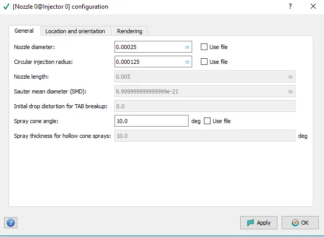
* All 4 nozzles are created with same above shown parameters, but the co-ordinates specifying the nozzle location is different for different nozzles. Nozzles are named as nozzle0, nozzle1, nozzle2, nozzle3.
Co-ordinates and align vector for all 4 nozzles are shown below,
1. Nozzle 0
- center 0.0823357 0.00100001 0.07019
- Align Vector -0.732501 0.210489 -0.647408
2. Nozzle 1
- center 0.0823357 -0.00099999 0.07019
- Align Vector -0.732501 -0.210489 -0.647408
3.Nozzle 2
- center 0.0823357 -0.0004 0.07019
- Align Vector -0.5 -0.2 -0.647408
4. Nozzle 3
- center 0.0823357 0.0003 0.07019
- Align Vector -0.5 0.2 -0.647408
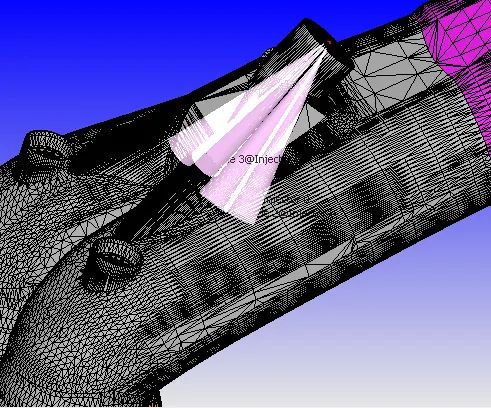
* After creating the nozzle, those can be seen in the engine geometry as shown below,
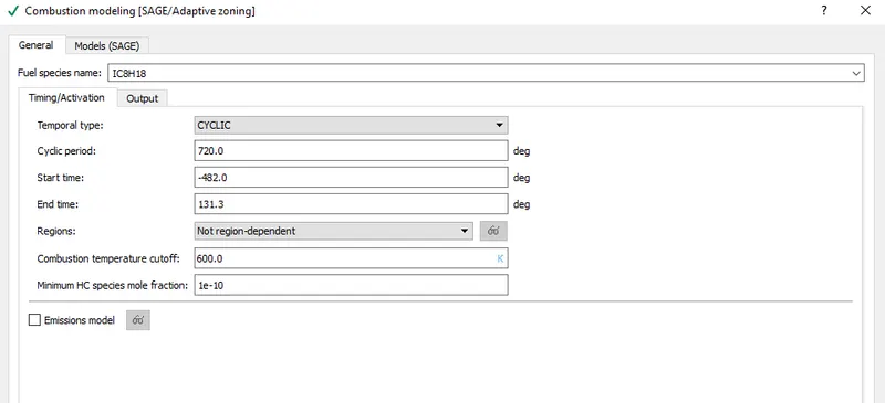
* Next important thing is setting up the combustion model, Under general parameters the start time, end time and cyclic period are set.
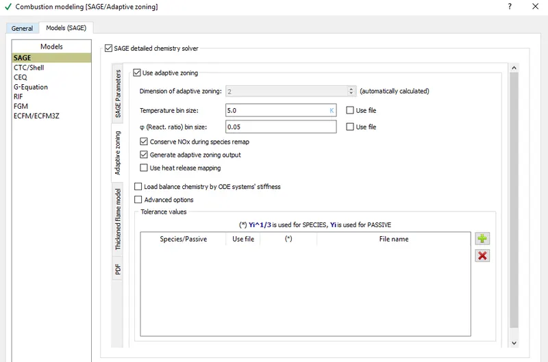
* SAGE model is used to simulate the combustion inside the engine. There are certain local controls under this which are left default. A snip of the same is provided below,
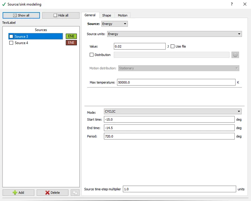
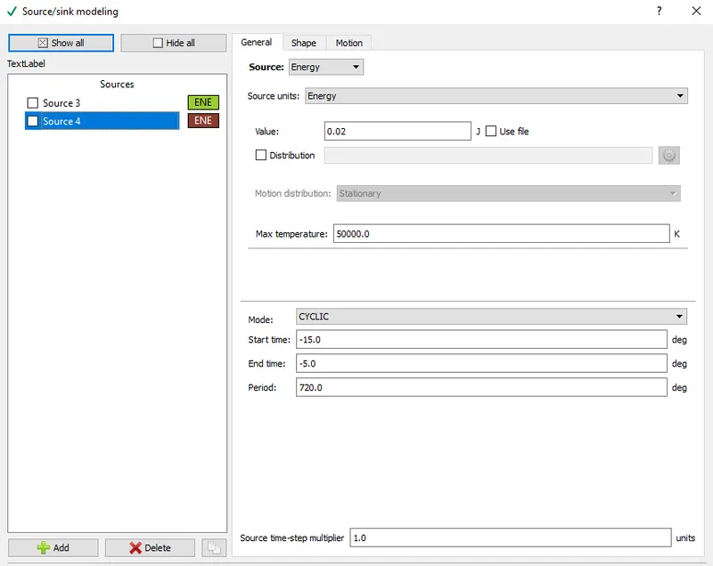
* Two energy source's are modelled so as to facilitatae the spark.
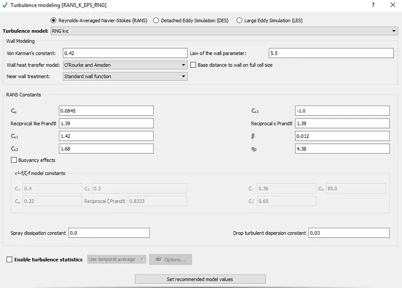
* For capturing turbulence RNG K-ε model is selected.
* A base grid size of 0.004 m is set, with adaptive mesh refinements. AMR setup is disscussed below.
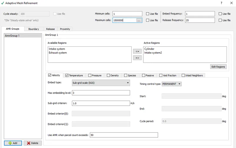
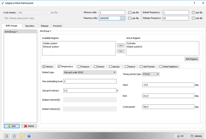
* AMR is applied for cylinder region and intake system2 region. Velocity as well as temperature based AMR is applied. For velocity based AMR max embedding scale of 3 and sub grid criterion of 1.0 is applied and timing control type is set to permanent and for temperature based AMR max embedding level of 3 and sub grid criterion of 2.5 is applied and timing control type is set to cyclic with start time of -17 degree and end time of 131 degree. Maximum cell of 1500000 is set.
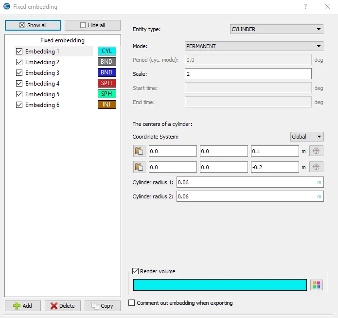
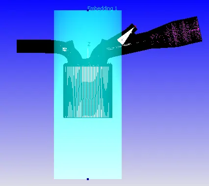
* Total of 6 fixed embedding's were applied, which are disscussed as below.
* A cylinder embedding ia applied such that it covers the cylinder region and a part of intake and exhaust region. A embedd scale of 2 is applied. A snip of the same is provided below,
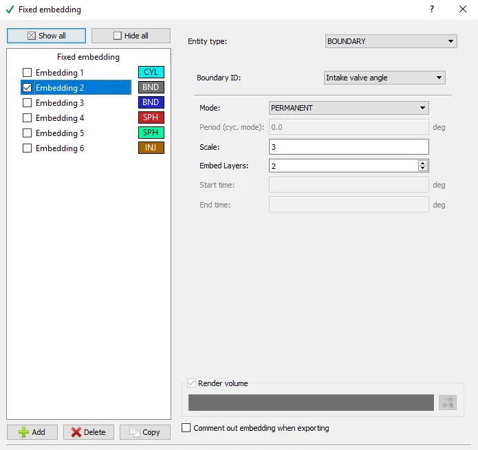
* A boundary embedding is applied on intake valve angle with a embedd scale of 3 and number of embedd layers set at 2.
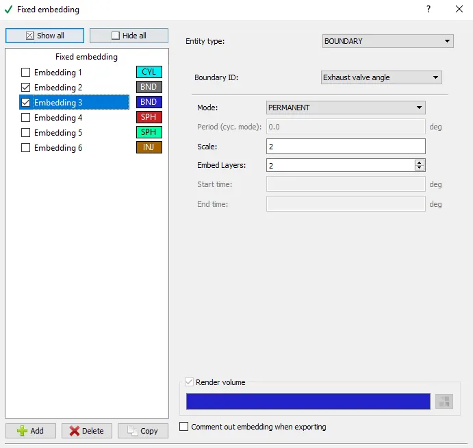
* Similarly a boundary embedd is applied on exhaust valve angle with a embedd scale of 2 and number of embedd layers set at 2.
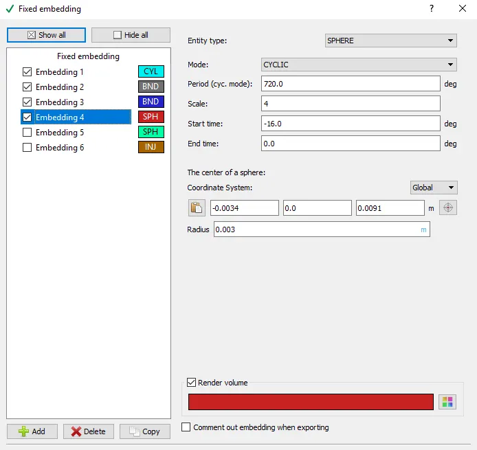
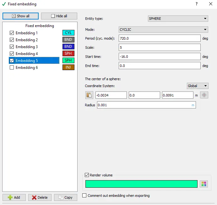
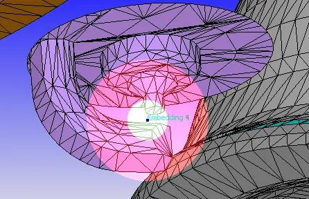
* 2 spherical embedding were applied at the spark plug electrode with a embedd scale of 4 and start time of -16 degree and end time of 0 degree, start time and end time needs to be specified since cyclic mode is selected. Same parameters were used while defining the two spherical embedd's only difference being in the radius of the embedd's. Snip of the same is shown below,
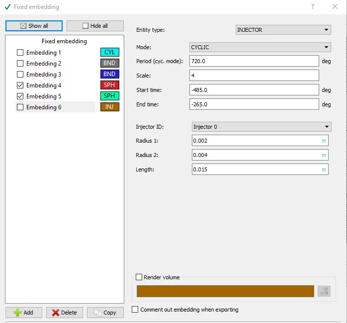
* Last is a injector embedd applied on the injector's. Converge provides this feature. A cyclic embedd is set with a period of 720 degree with start time of -485 degree and end time of -265 degree and with a scale of 4. Other details concerned with the embedding are radius and length which is as shown in the below snip,
* This completes the case setup, simulation is ran and results are noted.
* RESULTS AND OBSERVATIONS:
* Calculating Compression ratio: It is defined as ratio of max. volume/min. volume.
compression ratio, `r_c = (V_d + V_c)/V_c`
From the volume plot as shown below.
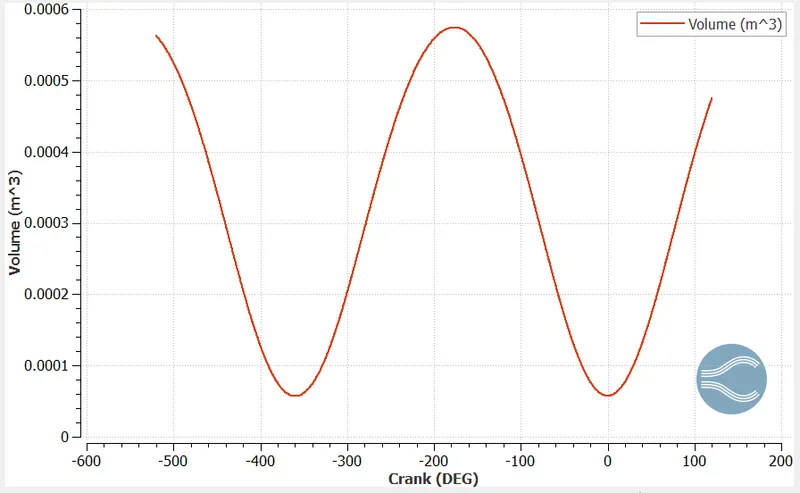
we have minimum volume at -360 deg, i.e, `V_c = 5.70311 * 10^-5 m^3`
also we have maximum volume at -176.35 deg i.e, `V_d + V_c = 0.000574218 m^3`
therefore compression ratio, `r_c`= 0.000574218/(5.70311e-05) = 10.068
* Calculating the combustion efficiency of the engine: It is defined as ratio of energy released by the burnt fuel to and the theoretical energy content of the fuel mass during one complete engine cycle.
It is given as `eta_c = (H_r - H_p)/(m_f*Q_(hv))`
where `H_r -` entalphy of reactant (J)
`H_p -` entalphy of product (J)
`Q_(hv) -` lower heating value of fuel mass (J)
As far as simulations are concerned the numerator part is calculated using the integated heat release plot, as shown below
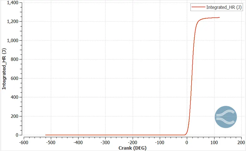
from the above plot we have integrated_HR = 1241.04 J
Lower heating value of `iC_8H_18`= 44.651 MJ/kg.
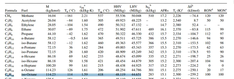
mass of fuel injected per cycle = 3e-05 kg
therefor heat generated per cycle = 3e-05*44.651*e06 J
= 1339.53 Joules
`eta_c = 1241.04/1339.53*100 = 92.64 %`
* Calculating power and torque of the engine:
Workdone by an engine is given by the formula, `w = T*theta`
where w - workdone (N-m, J)
T - torque (N-m)
`theta -` rotation angle (radians)
from engine performance calculator we have workdone , w = 468.646 N-m
therfore torque, T = w/`theta`
`theta`= 240.199 degree, Duration for which workdone is calculated (obtained from engine performance calculator)
Torque, T = 468.646/4.192106 = 111.7924 N-m
Power, `P = (2*pi*N*T)/60`
P - power (J/s)
N - engine speed (rpm)
T - torqu (N-m)
therfore Power, P = 2*`pi`*3000*111.7924/60 = 35.120 KJ/s
OR
we have Power given as P = Workdone/time
we have engine speed given as 3000 rpm, i.e 3000 rotation for 60 sec
so 1 rotation = 360 degree, so 360*3000 degree of rotation for 60 sec, from this we can calculate time taken in second for rotating 1 deg = 60/3000*360 = 5.55e-05 sec/deg
from the engine performance calculator we have the duration (in degree) for which the workdone is calculated which is = 240.199 degree.
so time taken for rotating 240.199 degree = 240.199*5.55*e-05 = 0.01333 sec.
therefore Power, P = 468.646/0.01333 = 35.236 KJ/sec
P = 2*`pi`*N*T/60 from this we have torque,
T = P*60/(2*`pi`*N) = 35.236e03*60/(2*3.14*3000) = 112.14 N-m
Power and torque can be calculated anyway around, which approximates to almost same answer.
* Engine performance calculator is a tool that can be used to calculate engine power, imep etc of the engine. Thermo_0 file for the cylinder region is used to calculate the engne power and imep. A snip of the same is given below,
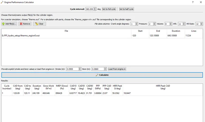
* In the above engine performance calculator we can find CAD10, 50 and 90 these represents the crank angle at which 10%, 50% and 90% of combustion has taken place, physical significance of CA10 is that it is used to identify the start of ignition of fuel present in the engine whereas CA50 indicates the end of premixed combustion and start of diffusion combustion of the fuel used in the engine. CA90 signfies the end of diffusion combustion.
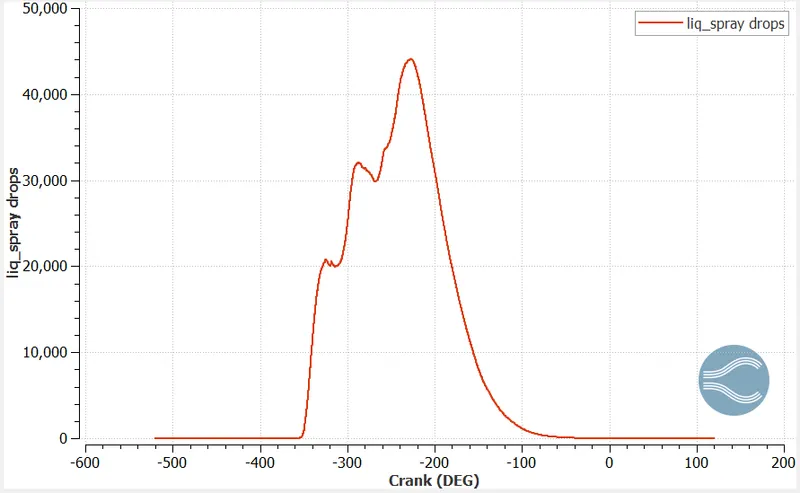
* Parcel count at cylinder region:
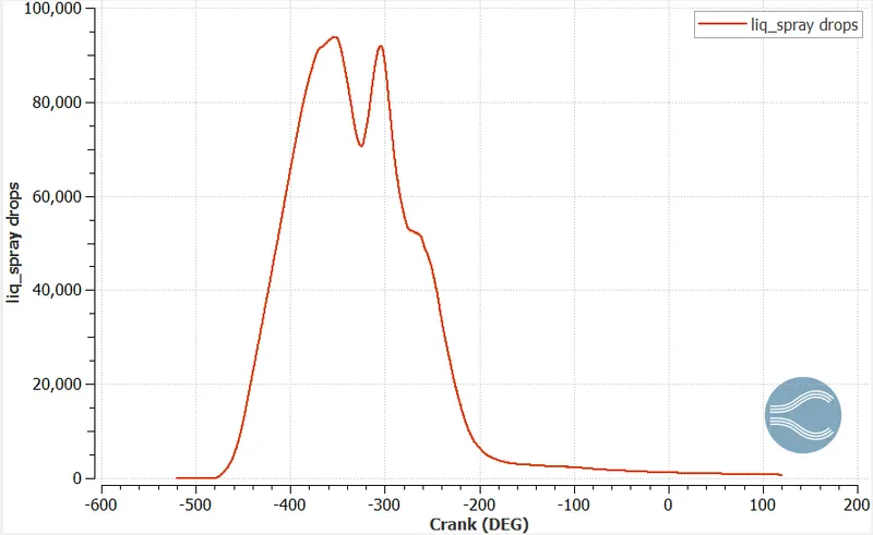
* Parcel count at intake system2 region:
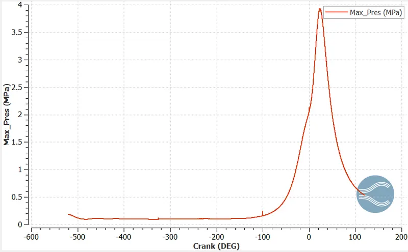
* Max pressure attained in the cylinder region:
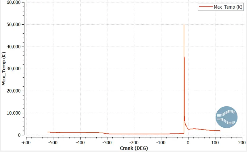
* Max temperature attained in the cylinder region:
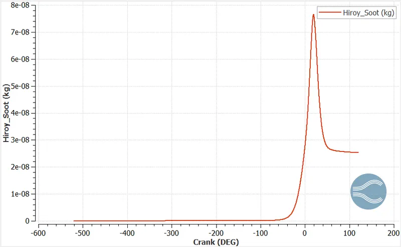
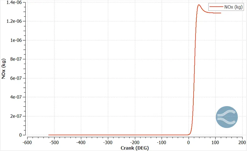
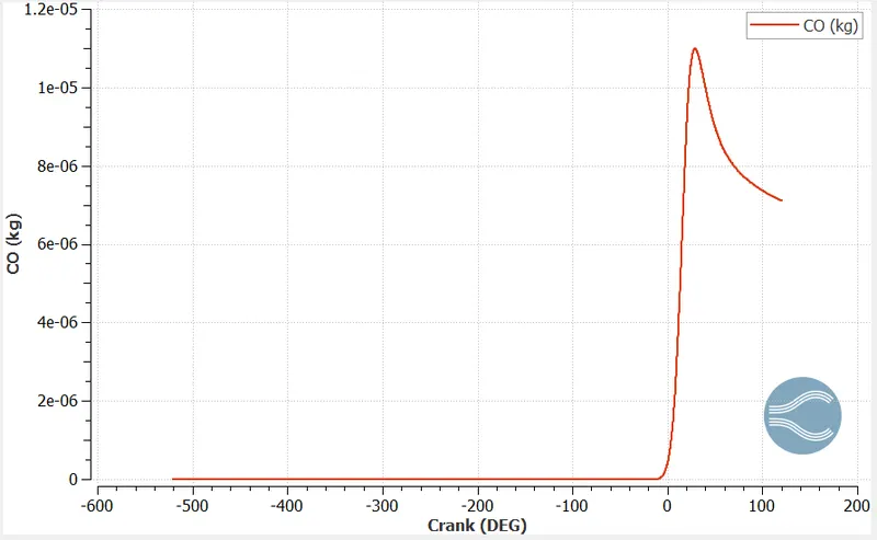
* Similarly we can check the different pollutant formation in any of the region. Since our interest is in the pollutants formed in the cylinder region it is being observed,
* Soot formation in the cylinder region:
* No_x formation in the cylinder region:
* CO formation at cylinder region:
* Flame propagation animation:
* Velocity animation:
* In this a wall heat transfer model is used to determine the temperature distribution on the wall, reason for the same is to save the computational time. To run the transient simulation in an ic engine along with combustion and reaction it takes too much time and hence determining the wall heat transfer (or to determine temperature distribution) along with these calculations will be too much time consuming, to compensate for this a wall heat transfer model is used.