Week 7 - Auto ignition using Cantera

AIM

* Plot the variation of autoignition time of methane with a constant temperature of 1250 K and pressure varying from 1 to 5 atm.

* Plot the variation of auto ignition time of methane with a constant pressure of 5 atm and temperature varying from 950 K to 1450 K.

* Further observe and print the rate of change of molar concentration of `H_2O, O_2, OH`w.r.t simulation time = 10 sec

-- When temperature is 1000 K and pressure is 5 bar.

-- When temperature is 500 K and pressure is 5 bar.

INTRODUCTION

Auto ignition temperature or kindling pont of a substance is the lowest temperature in which it spontaneously ignites in a normal atmosphere without an external source of ignition. At a given temperature. Autoignition time delay is defined as the time for which a homogenous mixture must be maintained at temperature T and pressure p before it autognites. This can be better explained by taking example of gasoline, the autoignition temperature of gasoline is about 553 K, so for a given amount of gasoline at room temperature if we increase its temperature to autoignition temperature of 553 K, even after attaining 553 K it will take some time for the gasoline mixture to combust, that small delay is called ignition delay time and it is in milliseconds.

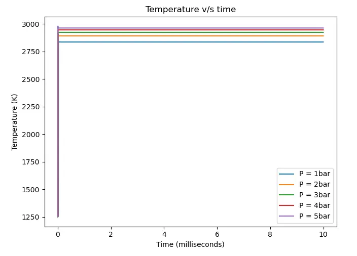
Practically this time is calculated from the temperature v/s time plot, it is given as `Time_(ignd) = Time_(i + 400 k)` , i.e time at temperature equals to initial temperature + 400 K.

To achieve the above targets cantera is used. In cantera we use the function called reactor. Reactor is the simplest reacting mechanism that can be defined in cantera. In here we use the methane and air as the gas mixture, as stated above the ignition time delay is in milliseconds and to capture this, reacting system needs to be taken from one state to other in milliseconds.

Reactors in cantera define the equations that need to be solved so as to take the air-fuel mixture from one state to another, but without a reactor network the system of equations cannot be solved. In other words even if there is a single reactor to take it from one state to another there has to be a reactor network which integrates the flow equations defined in the reactor.

It can be illustrated as follow,

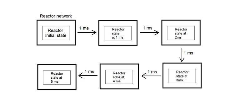
Logic :

* First the fuel-air mixture needs to be defined, in here the methane-air is taken, the stoichometric combustion equation is defined as

`CH_4 + 2*(O_2+3.76N_2) = CO_2 + 2H_2O+7.52N_2`

* Once the fuel-air mixture is fixed, its initial state needs to be defined using .TPX function. For 1st case where the variation of ignition delay time is plotted against varying pressure the temperature is held constant in .TPX function and for 2nd case the pressure is held constant and temperature is varied in .TPX function.

* Defined air-fuel mixture has to be inserted into a reactor, cantera provides different reactors such as ConstPressureReactor, FlowReactor, IdealGasConstPressureReactor, IdealGasReactor. For this challenge IdealGasReactor is used.

r = ct.IdealGasReactor(gas)

Above command creates a reactor r for which the gas is given as input.

* As stated in the introduction part, for the reactor to integrate its flow equations a reactor netwrok is required, the ReactorNet function of cantera is used for the purpose and the above defined reactor is given as input for the same.

sim = ct.ReactorNet([r])

* Once the reactor network is defined next step would be advance it through small time intervals. It is provided that the simulation needs to be carried for 10 sec, i.e 10000 milliseconds. A for loop in range of 10000 is defined and a initial time of 1 millisecond, advance function of cantera is used. After each iteration the time is increased by 1 millisecond.

sim.advance(time)

* A instance of SolutionArray class is created and a extra variable time is created,

states = ct.SolutionArray(gas, extra=['time'])

* For each iteration of the for loop the states object is appended with thermodynamic state of the reactor along witht the time is updated, following command line serves the purpose.

states.append(r.thermo.state, time=time)

* To print the ignition delay time the interp function of the numpy module is used.

If we consider a x,y plot for a given value of x if we have to find out the value of y interpolation is the means by which we can achieve this, the interp function of the numpy module does the same.

y_value = np.interp(x_value,x,y)

Suppose for the same x,y plot if we need to find out the x value for a given y value then the above command can be written as

x_value = np.interp(y_value,y,x)

Same logic is being used in computing the ignition delay value from plot of (time (x), temperature (y)) plot.

* Variation of autoignition time of methane with a constant temperature of 1250 K and pressure varying from 1 to 5 atm :

"""
Variation of autoignition delay with pressure
"""
import sys

import numpy as np

import cantera as ct

import matplotlib.pyplot as plt

gas = ct.Solution('gri30.xml')

a = [1,2,3,4,5]

P = [] # Defining an empty array for pressure values

ign_time = [] # Defining an empty array for ignition time

states = []

for i in range(0,5):

	P.append(a[i]*101325)

	T = 1250 # Defining a initial temperature in K

	gas.TPX = T,P[i],{'CH4':1,'O2':2,'N2':7.52}

	r = ct.IdealGasReactor(gas)

	sim = ct.ReactorNet([r])

	time = 0.0

	states = ct.SolutionArray(gas, extra=['time'])

	for n in range(10000):

		time += 1e-3

		sim.advance(time)

		states.append(r.thermo.state, time=time)

		
	plt.plot(states.time, states.T)
	plt.xlabel('Time (milliseconds)')
	plt.ylabel('Temperature (K)')
	plt.title('Temperature v/s time')
	plt.legend(["P = 1bar","P = 2bar","P = 3bar","P = 4bar","P = 5bar"])
	

	y_value = 1650

	x_value = np.interp(y_value,states.T,states.time)

	print(x_value)

	ign_time.append(x_value)


plt.show()

plt.plot(P,ign_time)
plt.xlabel('pressure (Pa)')
plt.ylabel('Ignition delay time (milliseconds)')
plt.title('Pressuer v/s Ignition delay')
plt.show()

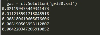
* Ignition delay time for increasing pressure :

* Temperature v/s time plot :

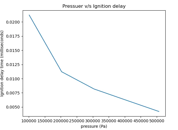
* Plot of variation of ignition delay time with increasing pressure:

* Variation of auto ignition time of methane with a constant pressure of 5 atm and temperature varying from 950 K to 1450 K.

"""
Understanding reactor network for auto ignition calculations
"""
import sys

import numpy as np

import cantera as ct

import matplotlib.pyplot as plt

gas = ct.Solution('gri30.xml')

T = [950,1050,1150,1250,1350,1450]

ign_time = [] # Defining an empty array for ignition time

states = []

for i in range(0,6):

	gas.TPX = T[i],5*101325,{'CH4':1,'O2':2,'N2':7.52}

	r = ct.IdealGasReactor(gas)

	sim = ct.ReactorNet([r])

	time = 0.0

	states = ct.SolutionArray(gas, extra=['time'])

	for n in range(1000):

		time += 1e-3

		sim.advance(time)

		states.append(r.thermo.state, time=time)

		
	plt.plot(states.time, states.T)
	plt.xlabel('Time (milliseconds)')
	plt.ylabel('Temperature (K)')
	plt.title('Temperature v/s time')
	plt.legend(["T = 950 K","T = 1050 K","T = 1150 K","T = 1250 K","T = 1350 K","T = 1450 K"])
	

	y_value = T[i] + 400

	x_value = np.interp(y_value,states.T,states.time)

	print(x_value)

	ign_time.append(x_value)


plt.show()

plt.plot(T,ign_time)
plt.xlabel('Temperature (K)')
plt.ylabel('Ignition delay time (milliseconds)')
plt.title('Temperature v/s Ignition delay')
plt.show()

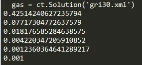
* Ignition delay time for increasing temperature :

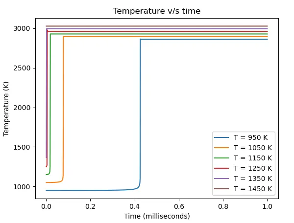
* Temperature v/s time plot :

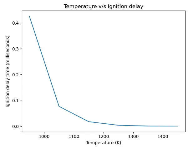
* Plot of variation of ignition delay time with increasing temperature:

* To print the rate of change of molar concentration of `H_2O, O_2, OH` w.r.t simulation time = 10 sec :

--> When temperature is 1000 K and pressure is 5 bar.

"""
Varition of molar concentration of H2O, O2, OH at 5 bar and 1000 K
"""
import sys

import numpy as np

import cantera as ct

import matplotlib.pyplot as plt

gas = ct.Solution('gri30.xml')

T = 1000 # Defining a initial temperature in K

P = 5*101325 # Definiing initial pressure of 5 atm

gas.TPX = T,P,{'CH4':1,'O2':2,'N2':7.52}

r1 = ct.IdealGasReactor(gas)

sim = ct.ReactorNet([r1])

time = 0.0

states = ct.SolutionArray(gas, extra=['time'])

for n in range(10000):

	time += 1e-3

	sim.advance(time)

	states.append(r1.thermo.state, time=time)

print('Molar concentration of H2O = ',states.X[:,gas.species_index('H2O')])
print('Molar concentration of O2 = ',states.X[:,gas.species_index('O2')])
print('Molar concentration of OH = ',states.X[:,gas.species_index('OH')])

* Molar concentration of different species at 5 bar and 1000 K :

--> When temperature is 500 K and pressure is 5 bar.

"""
Varition of molar concentration of H2O, O2, OH at 5 bar and 500 K
"""
import sys

import numpy as np

import cantera as ct

import matplotlib.pyplot as plt

gas = ct.Solution('gri30.xml')

T = 500 # Defining a initial temperature in K

P = 5*101325 # Definiing initial pressure of 5 atm

gas.TPX = T,P,{'CH4':1,'O2':2,'N2':7.52}

r1 = ct.IdealGasReactor(gas)

sim = ct.ReactorNet([r1])

time = 0.0

states = ct.SolutionArray(gas, extra=['time'])

for n in range(10000):

	time += 1e-3

	sim.advance(time)

	states.append(r1.thermo.state, time=time)

print('Molar concentration of H2O = ',states.X[:,gas.species_index('H2O')])
print('Molar concentration of O2 = ',states.X[:,gas.species_index('O2')])
print('Molar concentration of OH = ',states.X[:,gas.species_index('OH')])

* Molar concentration of different species at 5 bar and 500 K :

Observations :

* At a constant temperature of 1250 K as the pressure is increased from 1 bar to 5 bar the autoignition delay gets reduced.

* At constant pressure of 5 bar as temperature is increased from 950 K to 1450 K, autoignition delay gets reduced. Until a temperature is reached the reduction in the autoignition delay is drastic after which it is alsmost constant.

* At constant pressure of 5 bar as the temperature is decreased from 1000 K to 500 K, molar concentration of `H_2O`gets decreased from 1.65670203e-01 to 1.58442591e-16, molar concentration of `O_2`gets increased from 0.01245913 to 0.19011407, molar concentration of `OH` gets decreased from 1.30328522e-02 to 2.65566188e-23. Hence overall we can say that at constant pressure decreasing the temperature of methane-air mixture reduces the molar concentration.