Week 1 : Exploring the GUI of GT-POWER
1. Different modules of GT-Power:
* Mechanical - Includes simulation of kinematics, multi-body dynamics, frequency domain.
* Electric and electromagnetic - Includes simulation of circuits, electromechanical devices.
* Flow - Simulation of fluid, gas, liquid or mixture.
* Acoustics - Simulation of linear and non linear.
* Thermal - simulation of all types of heat transfer.
* Chemistry - Includes simulating combustion using detailed chemical kinetics.
* Controls library for signal processing
2. Locate following settings:
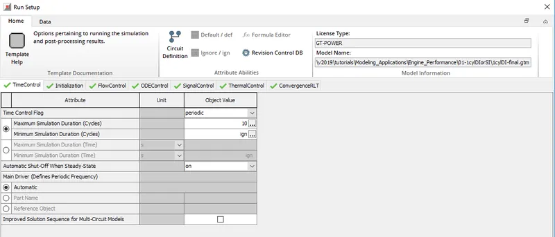
* Time control flag - This local control is found under run setup, using time control flag we can set maximum simulation duration and minimum simulation duration. A snip of the same is provided below,
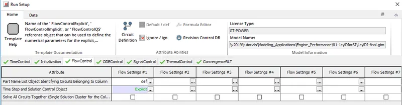
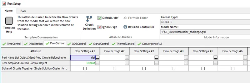
* Time step and solution control - This local control is found under the run setup as well, to be specific under flow control tab as an attribute. Using this attribute we can set the type of solver to be used to solve the flow equations. FlowControlExplict, FlowControlImplicit, Flowcontrol QS are the options available.
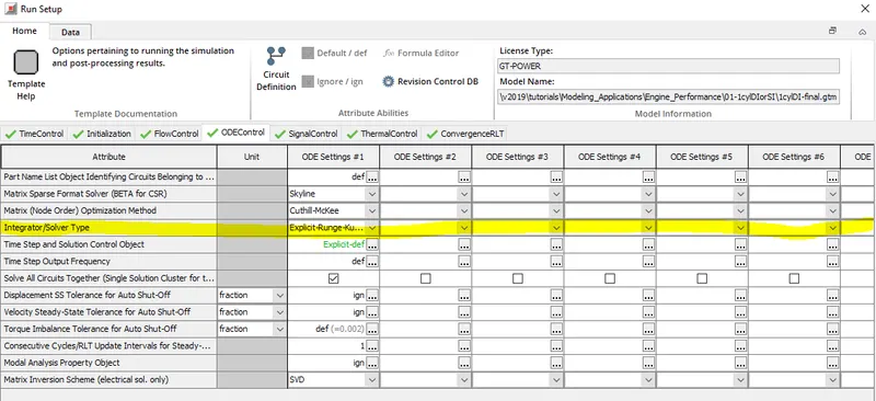
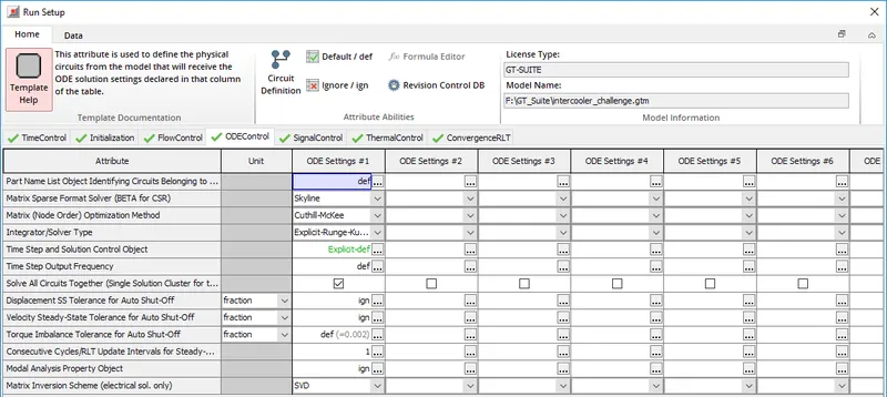
* Integrator/solver type - This local control is found under the run setup, under ODE control tab as an attribute. Using this we can set the integrator/solver that can be used while time marching. There are several integrators available such as Explicit-Adams-PECE, Explicit-Runge-Kutta, Implicit-Trapezoidal, Implicit-H.H.T, Implicit-Radau2 etc. Each of these integrators are of different order of accuracy.
3. To explore intercooler tutorial and note down following changes :
* Run setup - Since intercooler is not like IC engines which works on cycles hence the simulation time is mentioned in seconds. Maximum simulation duration is given as 0.5 sec also the automatic shut off when steady state is achieved is turned on. This will end the simulation run as soon as the steady state is reached, if this attribute is tuned off then the simulation will run till the end time.
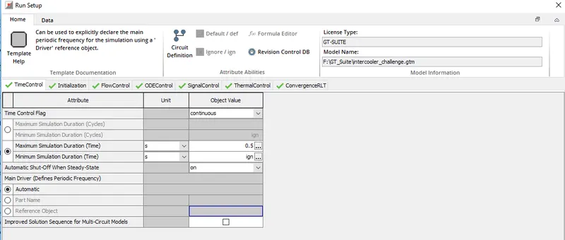
As far as the time step and solution control is concerned a explicit solver is used to run the simulations. Runge-kutta explicit integrator/solver type is used for time marching.
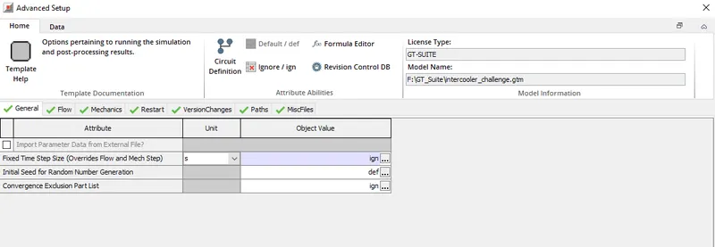
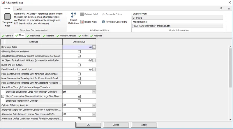
* Advanced setup - Most of the attributes under this local control is ignored and some are set to default.
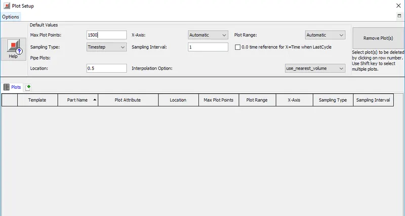
* Plot setup - Max number of points to be taken for plots is fixed at 1500. The x-axis and y-axis range's are set to automatic. For the templates to be active we need to activate some of the plots before running the simulatons.
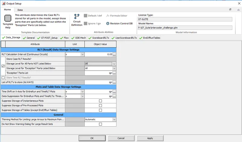
* Output setup - It has all the output setup concerned with plots, data storage etc. One of the important attribute that comes under data storage is RLT calculation interval. This interval determines how often RLT dependence reference objects are updated. For turbocooler modelling it is set at 0.05 sec. All the case results concerned with RLT are stored.
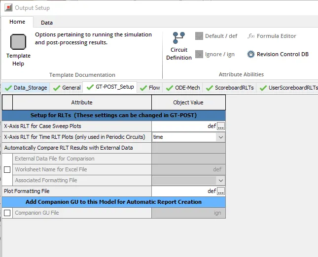
Time step plot is checked, also the supress .brf file is checked. All other attributes are ignored except X-axis RLT for casesweep plots which is set default. Plot formatting file is also set default.
4. To run a simulation on turbocahrger model with below attributes and hence compute the pressure drop across CAC, and heat transfer rate asross CAC :
Diameter of cooler inlet and outlet pipe = 50 mm
Length of the CAC = 1000 mm
Inlet mass flow rate = 1200Kg/hr at 100 deg C
Outlet pressure 2 bar at 30 deg C
* Intercooler tutorial is opened as a new project and it should be saved in a different directory with .gtm extension. The tubocharger model opened looks as follow,

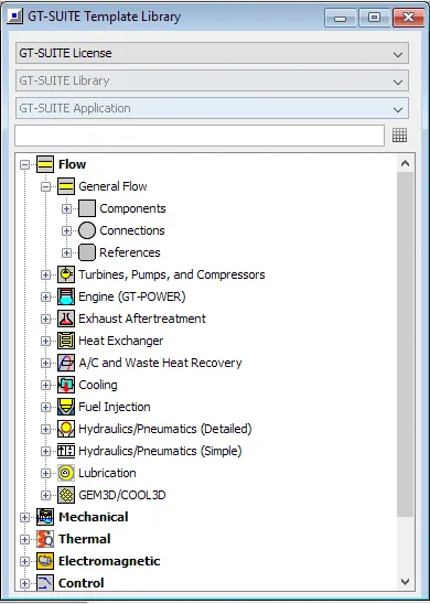
All the components seen in the above model is called a part. Each part belong to a object and the objects that represent a part or set of parts belong to a template. All the above shown parts can be fetched from the template library and can be used in the project map. A snip of the template library is as shown below,
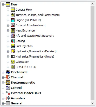
As it is seen from the above for flow parameter there are different templates available. Each template has sub templates such as components, connections, references etc. A snip of the same is shown below,
* A intercooler is used in a turbocharged or supercharged engines to reduce the temperature of compressed air and hence increase the oxygen content. The air at high temperature flows through the inlet of the intercooler, which consists of several pipes of equal size. As the high temperature air passes through the pipes the heat gets conducted into the pipes also the heated pipes are cooled by blowing air around the pipes.
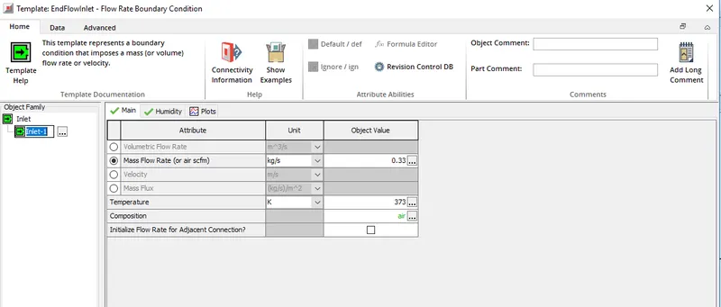
* In the above shown intercooler model Inlet-1 represents the outlet of the turbocharger compressor where the temperature of the air will be high. Inlet-1 belongs to inlet object which inturn belongs to the endflow inlet template. By double clicking on the part in the project map or template tree we can check the different attributes concerned with the high temperature air flowing out from the turbocharger. Mass flow rate, temperature of the fluid, and fluid composition can be set.
It is provided that inlet mass flow rate is 1200Kg/hr at 100 deg C,
Mass flow rate in Kg/s = 1200/3600 = 0.33 Kg/s
Temperature = 273 + 100 = 373 K, since the fluid is air the fluid composition is set as air. A snip of the attributes and value's set for the same is shown below,
* As far the attributes under the humidity tab is concerned those are ignored and no plots are checked as such.
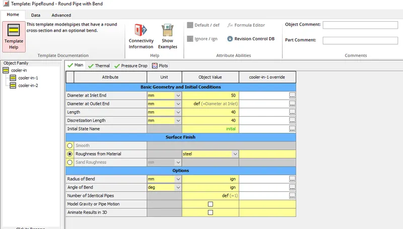
* Next comes the part cooler-in-1, It represents the inlet pipe, it belongs to the object cooler-in which inturn belongs to template cooler.
Inlet and outlet diameter of 50 mm is set as provided. The length and discretizaton length both are left as default values of 40 mm. Pipe material is selected as steel.
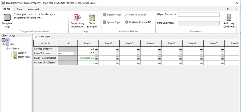
* Under the thermal tab we can set different attributes concerned with walls of the solid pipe. Object value of the wall layer properties object is by default set as inlet, double clicking on the object value inlet opens up another window where we can set attributes such as layer material, layer thickness, layer emissivity etc. A snip of the same is provided below along with all the attributes set.
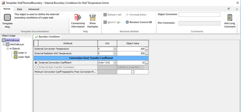
* Another attribute that is found under the thermal tab is wall external boundary condition object, for which the object value is inlet wall layer. By double clicking on the object value we can set attributes such as external convection temperature, external radiation sink temperature, external convection coefficient. All of these attributes are already set since intercooler model is fetched from tutorials and same value set is used. A snip of the same is provided below,
* Another part is cooler f-split 1, this connects the inlet pipe to the network of several pipes inside the CAC. Attributes under main tab are the volume, surface area and initial state name. Volume by default is set as 190000 mm^3 and is set as def. Initial state initialises the value of pressure, temperature and composition.
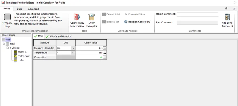
* For part cooler-1 and 2 as well as cooler f-split 1 and 2 the initial condition used are same. Initial pressure of 2.4 bar and temperature of 350 K is initialised.
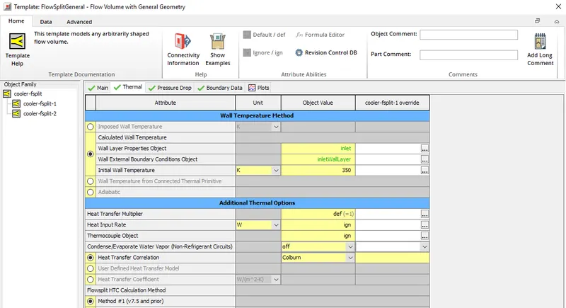
* Under thermal tab all the attributes set are same as the attributes set for the cooler in 1.
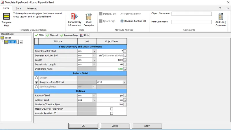
* Next is the important part which is the CAC itself. A round pipe template is used to represent the same. As mentioned above it consists of several equal sized pipes, number of pipes and the diameter of the pipe are attributes to be set. Pipe diameter is set as 7 mm and number of identical pipes is set as 100 along with the length set as 1000 mm.
* The pipes of the CAC exits as split, which is shown in the model as cooler f-split2, different attributes applied for this part is same as cooler f-split1. The splitted pipe joins the outlet pipe which is shown as cooler-in 2, different attributes applied are same as cooler-in 1.
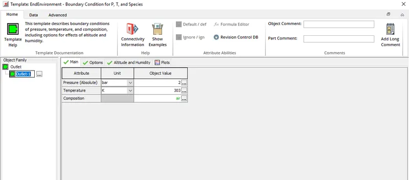
* Outlet-1 is the exit from where the low temperature air flows out. Outlet pressure is set as 2 bar at 303 K.
* Once all the above is set the case setup is run and the results are obtained. Results can be post-processed in the post processing tool GT-post. A snip of the post-processing window is shown below,
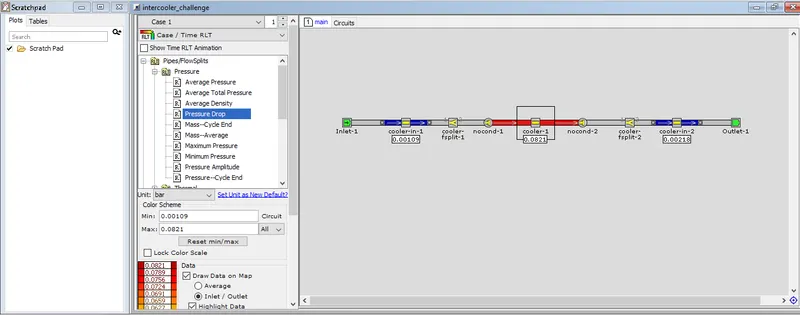
* Since our aim is to calculate the pressure drop and net heat transfer rates, these can be obtained using the result attributes.
* Pressure drop across CAC :
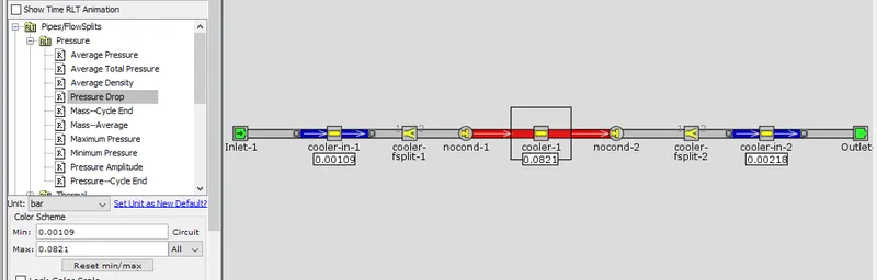
from the above snip it is clear that the max pressure drop is at CAC which = 0.0821 bar.
* Net heat transfer at CAC :
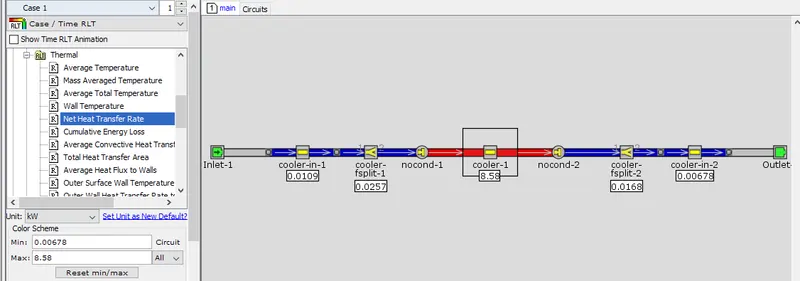
from the above snip the net heat transfer rate at CAC = 8.58 KW