Week 10: Modeling and Simulation of flow around an Ahmed Body
AIM
* To create a ahmed body model, along with the virtual wind tunnel and run a external aerodynamics simulation.
* To post-process the result obtained from simulation and plot velocity along vertical direction at different points in the flow path.
* To calculate the drag coefficient.
INTRODUCTION
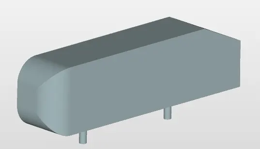
Ahmed body is a geometry which represents a generic car body. We can consider it as a blunt body which has a rough geometry resemblance that of a car, it was first developed and experimented by s.r Ahmed and hence it is named as ahmed body. Significance of an ahmed body is that, suppose we have developed a CFD code, which we need to run simulations around a new model car which is to be developed, so in that case we can use ahmed body to check whether the codes that were developed is good. We can use the codes and run simulations around a ahmed body to capture flow parameters in a turbulent flow. If we are able to validate the numerical results then we can use the codes to develop the new model car.
Below is a typical illustration of a ahmed body:
* In this challenge the dimensions for the ahmed body used are shown below,
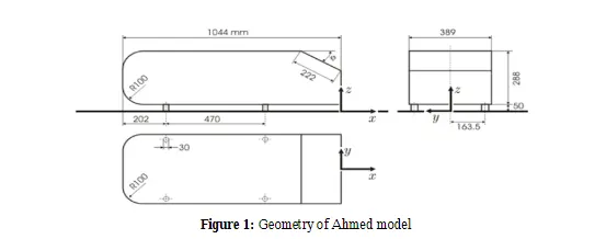
Slant angle of at hinde side of the ahmed body is set to 35 degree. The virtual wind tunnel is modelled using the following dimensions,
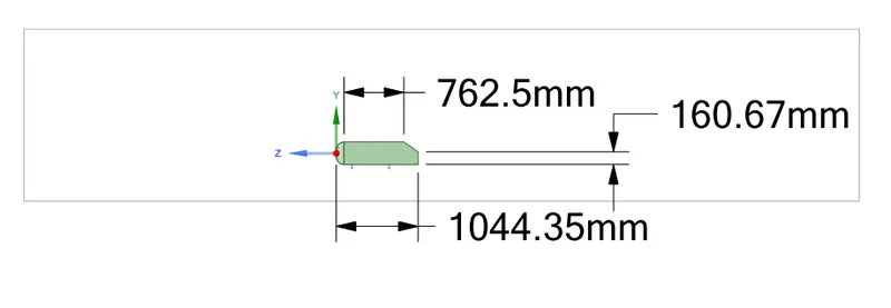
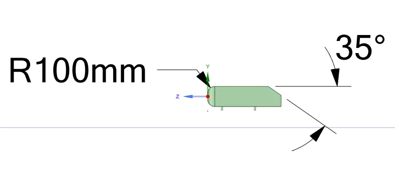
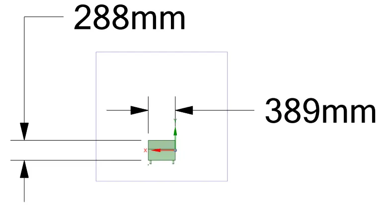
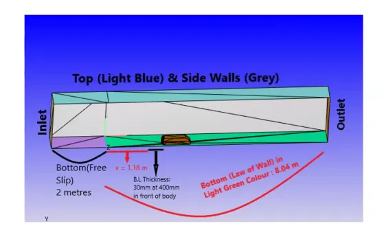
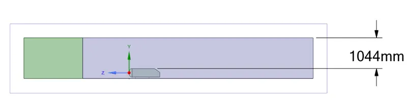
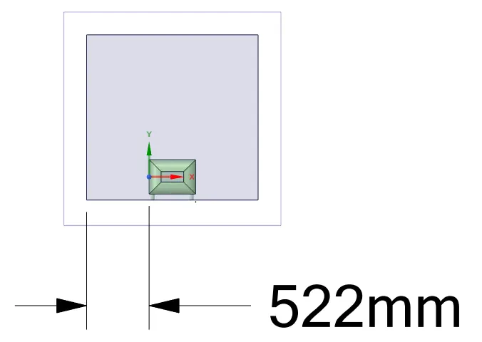
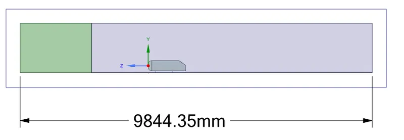
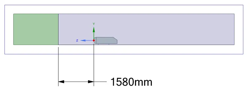
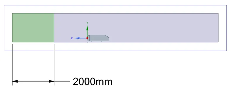
* While modelling the virtual wind tunnel, from the inlet upto a distance of 2 meter a slip boundary condition is provided. From the front of the ahmed body till the slip boundary wall a distance of 1.58 meters is maintained so that a 30 mm thick boundary layer is formed.
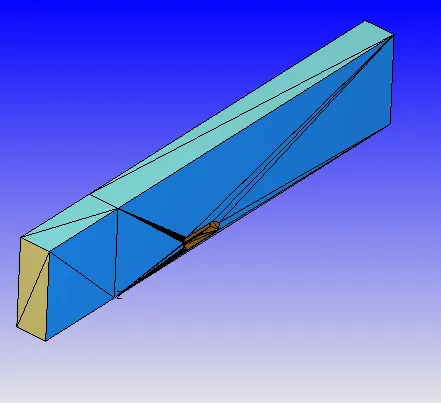
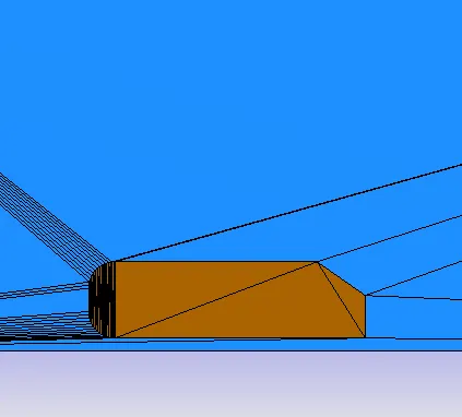
* After creating the entire geometry with above illustrated dimensions, the geometry is halved and one half of the geometry is used for the simulation. It is then opened in converge and a geometry clean-up is done so as to get away from all the possible errors. The completed geometry from converge is illustrated below,
Case steup:
* Materials for the gas simulation is set with deafult global transport parameters. `O_2`, `N_2` are the species set.
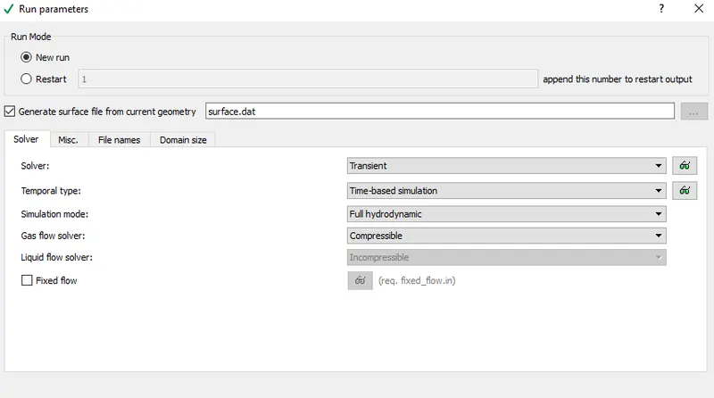
* Next comes the simulation parameters. Under run parameters a full hydrodynamic transient simulation with compressible flow is set. Other local controls under the run parameters are set to default values.
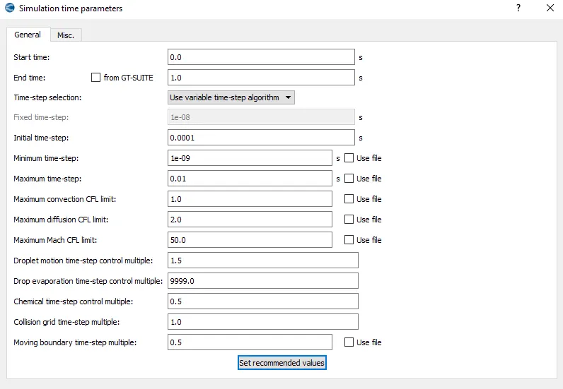
* Initial time is set to zero and final time is set to 1 with initial time step size of 0.0001 and minimum time step size of 1e-09 is set. Other local controls under the time parameters are set to default values.
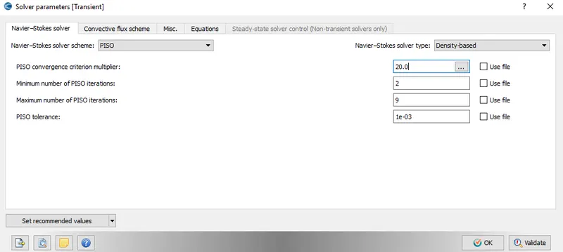
* Under solver parameters a density based solver type is set, since the flow is a compressible flow.
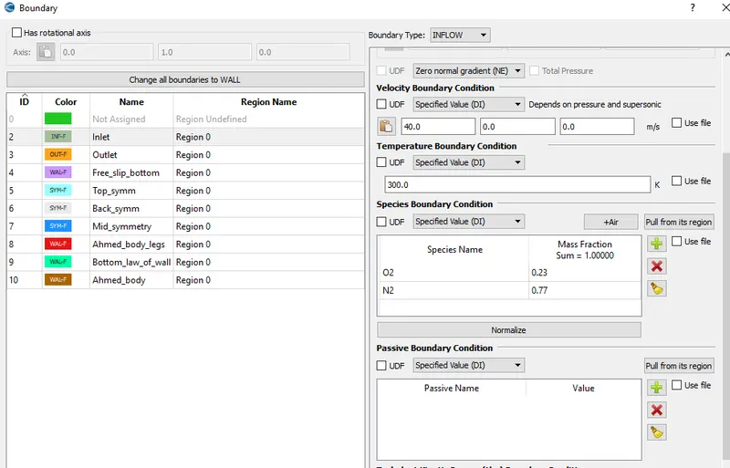
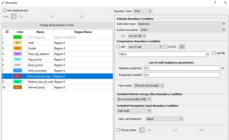
* A total of 9 boundary's are defined, boundary condition applied at each boundary are disscussed below,
1. Inlet : Inlet boundary condition is set to inflow type and a velocity of 40 m/s is defined. Both `O_2` as well as `N_2` are set as the species.
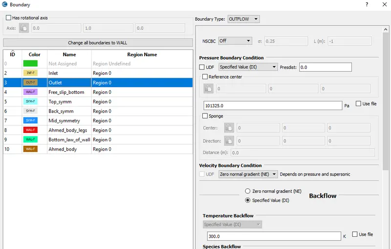
2. Outlet: For this the boundary type is set as outflow, atmospheric pressure of 101325 Pa is defined with `O_2` and `N_2` set as the species.
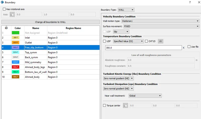
3. Free_slip_bottom: This is a 2 meter base wall from the inlet. Boundary type is set as wall, a stationary wall with slip boundary condition is defined.
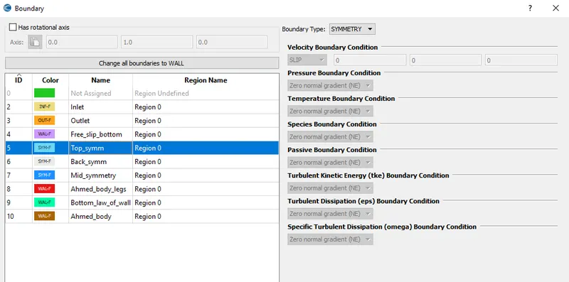
4. Top_symm: This is the top surface of the virtual wind tunnel, for this the boundary type is set as symmetry.
5. Back_symm: This is the back surface of the virtual wind tunnel, for whcih the boundary type is set as symmetry.
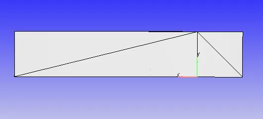
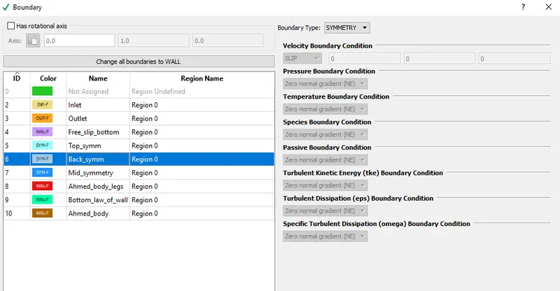
6.Mid_symmetry: This is the surface that cut's the ahmed body into 2 halve's, for which the boundary type is set as symmetry.
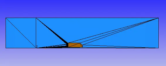
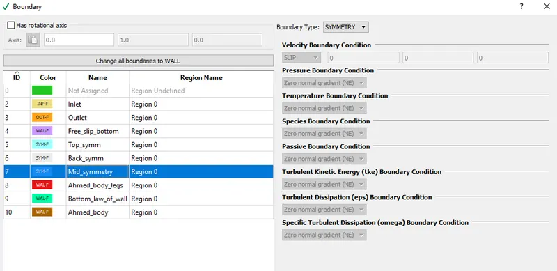
7. Ahmed_body_legs: These are the boundary for the two legs of the ahmed body. The boundary type is set as a stationary wall with law-of-wall set as the boundary condition.
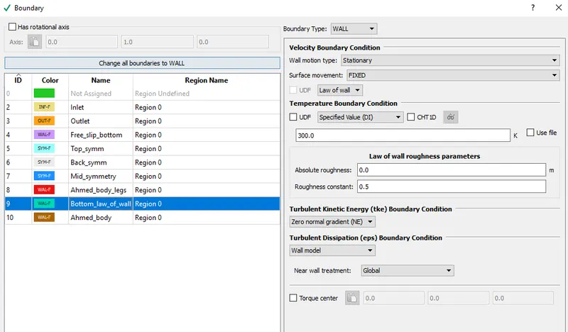
8. Bottom_law_of_wall: This is the surface after the 2 meter long no-slip wall, for this the boundary type is set as wall, a stationary, fixed wall with law-of-wall as the boundary condition.
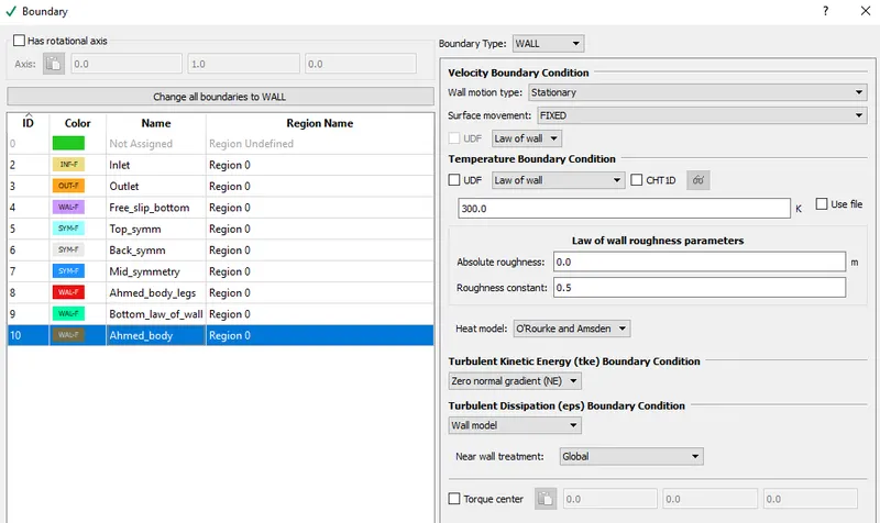
9. Ahmed_body: For this the boundary type is set as wall. A stationary, fixed wall with law-of-wall boundary condition.
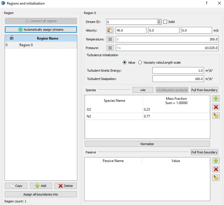
* Regions and initialization: The inlet velocity of 40 m/s is defined as the initial velocity and atmospheric pressure of 101325 Pa is defined as the initial pressure. Initial temperture is defined as 300 K. The region is labelled as region_0, each boundary are defined to this region_0.
* RNG K-`epsilon` is set as the turbullence model to capture the turbullence in the flow. Inflation layers are applied on the ahmed body using embedding.
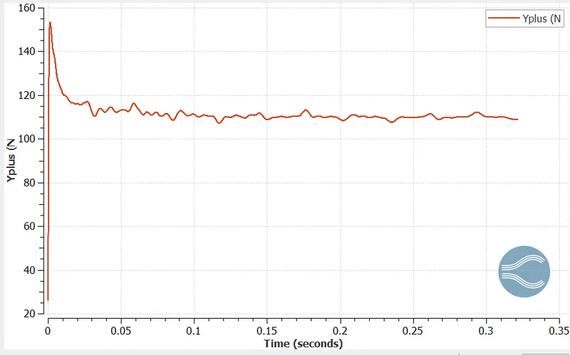
Since K-`epsilon` is the tubullence model used we can use y+ value ranging from 35 - 100. First layer thickness calculation is shown below,
`y+ = (rho*u_(tau)*y)/mu`
so from the above we can wirte, `y = (mu*(y+))/(rho*u_(tau))`
where, y is the first layer thickness
`u_(tau) = sqrt(tau_(w)/rho`
`tau_(w)` - Wall shear stress (N/m^2)
wall shear stress , `tau_(w) = 1/2*C_(f)*rho*V^2`
where, `C_(f)` - Skin friction
Skin friction, `C_(f) = 0.058*Re^-0.2`
`rho_(air) = 1.1765 (kg)/m^3`
`mu_(air) = 1.8538*10^(-5) (kg)/(m*s)`
Velocity of air, u = 40 m/s
Characteristic length of the ahmed body, L = 1.044 meter
Reynolds number, `Re = (u*L*rho)/mu`
`Re = (40*1.044*1.1765)/(1.8538*10^(-5)) = 2.6 * 10^(6)`
Skin friction, `C_(f) = 0.058*(2.6*10^(6))^(-0.2) = 0.0030`
Wall shear stress, `tau_(w) = 1/2*0.0030*1.1765*40^(2) = 2.823 N/(m)^2`
`U_(tau) = sqrt((2.823)/(1.1765)) = 1.549`
Since k-`epsilon` turbullence model is used y+ = 155 is used for first layer thickness calculations,
Therefore, First layer thickness, `Y = (1.8538*10^(-5) *155)/(1.1765*1.549) = 1.57 mm`
* Inflation layers are added using the embedd local control under the grid sizing option. In embedd layering the first layer thickness is calculated using the embedd level defined and the base grid size.
Grid size = Base grid / `2^n`
n - Embedd level
from our calculations we have first layer thckness, y = 1.57 mm
The base grid size is set to 20 mm
therefore, 1.57 = 20/`2^n`
calculating n from the above we get, n = 3.87.
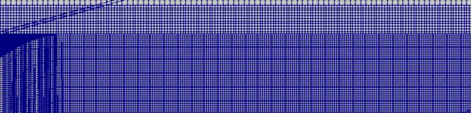
In converge we cannot mention the decimal number as embedd level and hence the embedd level is defined as 3, also a total of 10 embedd layers are defined. This completes applying the inflation layers or body fitted mesh around ahmed body.
Snip of the base grid defined as well as the embedd layer applied is shown below,
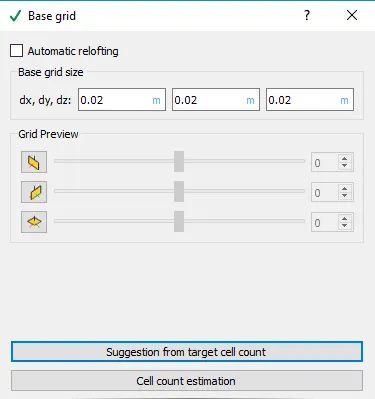
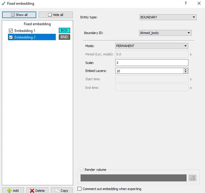
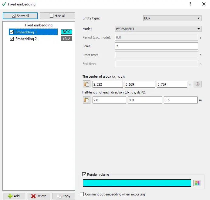
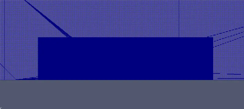
* One more embedding is applied around the ahmed body in box shape such that the cell size inside this embedd is much smaller than the base grid size. This embedd layer is just an analogy of density box. For defining the box we need to define the centre of the box as well as the half length in x, y and z direction. A snip of the defined values are as shown below,
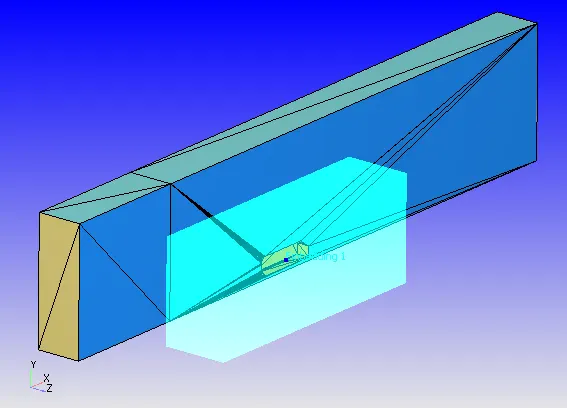
* When created the box embedd layer can be seen as shown below,
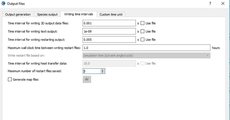
* Time intervals for writing the 3D o/p file as well as the text file are defined under the output/processing. A snip of the same is shown below,
* This completes setting up of the case and then the simulation is run using the cygwin and the results are post-processed using paraview.
* RESULTS OBTAINED
* Inflation layer:
* Box embedding:
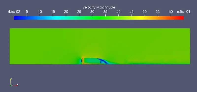
* Velocity contour:
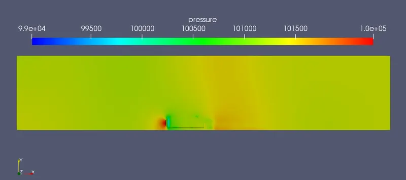
* Pressure contour:
* Y+ plot:
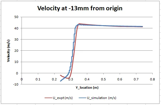
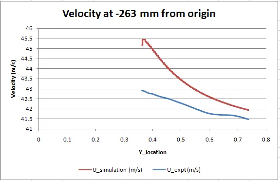
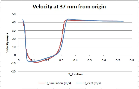
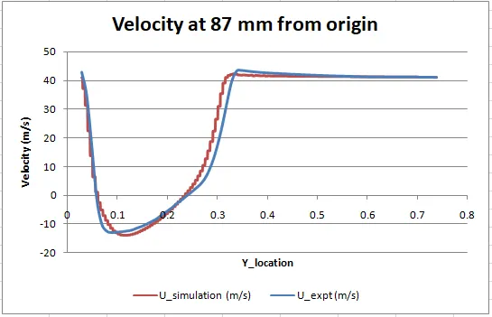
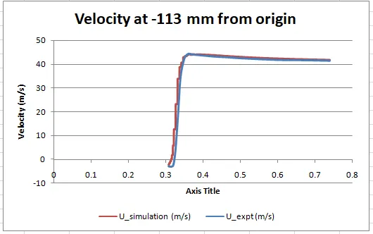
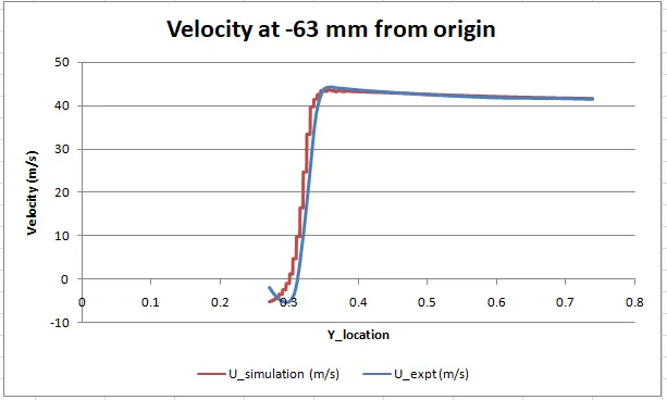
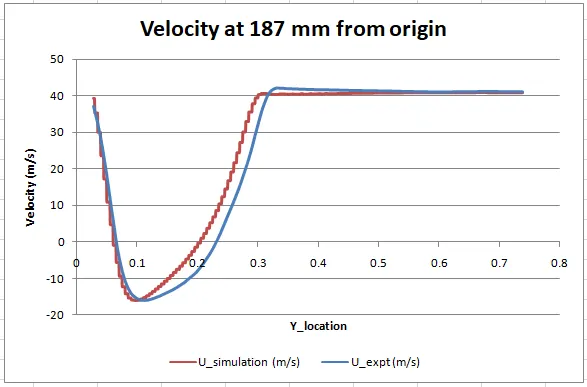
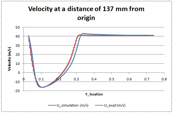
* The results obtained from the simulation is cross-checked with experimental results. In the external flow over ahmed body experiment different line probes are placed at different x-location (flow-direction) and velocity along the y-direction (direction perpendicular to the flow direction) are plotted. Different x-location at which the line probes placed are -13 mm, -263 mm, 37 mm, 87 mm, -113 mm, -63 mm, 187 mm, 137 mm from the origin.
* In paraview plot over line option is used and line probes are placed at above mentioned locations along x-direction and the velocity data obtained is plotted against the velocity data at same locations obatined from experimental results. Plots obtained are as shown below,
* Drag force and drag coefficient calculations:
Drag force is calculated from the P_x plot on ahmed body. The P_x plot is shown below,
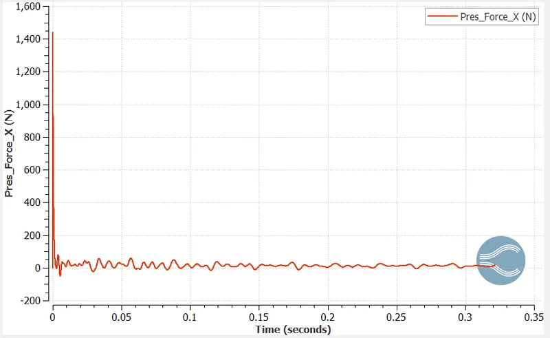
P_x data at all the time steps are extarcted and the average value is computed in the excel sheet which gives us P_x = 16.7 Newton.
hence Drag force, `F_d = 16.7 N`
* Drag coefficient is given as, `C_d = F_d/(1/2*rho*v^(2)*A)`
`F_d` - Drag force (N)
`rho` - Density of air (`(kg)/(m^3)`)
`v` - Inlet Velocity (m/s)
A - Frontal area (m^2)
`F_d = 16.7 N`
`rho = 1.1765 (kg)/m^3`
v = 40 m/s
Frontal area is calculated in paraview using some of the available local controls such as Extract block, Select cells on, Extract selection and integrate variables. A snip of the fontal area obtained from the paraview is shown below,
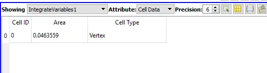
A = 0.04635 m^2
therefore, `C_d = 16.7/(1/2*1.1765*40^(2)*0.04635) = 0.382`