Week 6: Conjugate Heat Transfer Simulation
AIM
* To simulate Conjugate heat transfer analysis through a pipe.
* To run a grid dependence check.
* To explain briefly about supercycling and to run the simulation for different supercycle stage interval for base grid and hence note the simulation time.
INTRODUCTION
Conjugate heat transfer (CHT) refers to heat transfer process involving an interaction of conduction within a solid body and convection from solid body to fluid which is moving around the solid body. CHT analysis helps us to find out temperature distribution over solid surface, heat transfer coefficients. In this simulation a 2 pipe configuration geometry is used, which consists of a solid pipe of larger diameter enclosing another pipe of smaller diameter in which the fluid is flowing. Heat flux is supplied to the solid pipe this increases the temperature of solid pipe, heat is transffered from solid pipe to the fluid flowing through the inner pipe which is of low temperature through convection.
* Geometry:
As disscussed above the geometry used is of 2 pipe configuration as shown below,
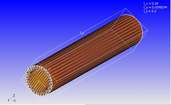
Geometry is created using the cylinder option which is under the create local control in the geometry dock of converge studio. While creating such a geometry the most common error that the diagnosis tool shows is that of intersection and Non-manifold errors. Intersection can be avoided by deleting the intersecting faces, once the intersecting faces are deleted we can create the face using loft edges and patch local controls. Non-manifold error cannot be avoided because in this type of 2 cylinder configuration geometry in more locations through the geometry one edge will be by 3 triangles. hence converge studio auto ignores Non-manifold error once we complete the other CHT case setup.
* Case setup:
* Under the material selection local control both gas and solid simulation is checked, reaction mechanism is unchecked and species is checked. A snip of the material selection local control is provided below,
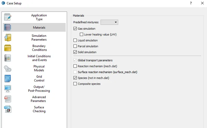
* Under materials local control there are 4 options viz gas simulation, solid simulation, global transport parameters, species. Upon these options gas simulation and global transport parameters is left as default. Under solid simulation tab Aluminium is selected as the solid material, this will be the material of outer solid pipe. O2 and N2 are the species added, those two will be the constituents of the air, the fluid flowing through the inner pipe.
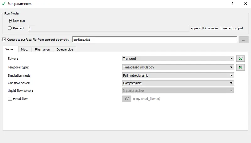
* Under Run parameter transient solver is selected, along with full hydrodynamic solving, gas flow solver is set as compressible. A snip of the same is provided below,
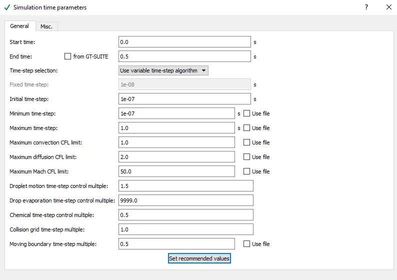
* Since the simulation is transient simulation time parameters are set in sec. start time is set to zero, end time is set to 0.5 sec, initial and minimum time step is set as 1e-7 and max time step is set as 1 sec. Max convection CFL limit is also set to 1.
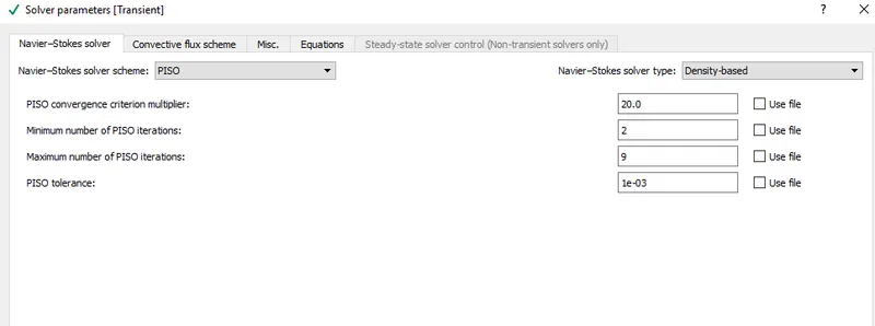
* Under solver parameter the solver type is set as density based solver, since the flow type is set as compressible in the Run parameter, density based solver is best suited to solve compressible flows. Under the equations tab the max iteration for the pressure is set as 5000. If the max iteration is not set, few seconds after running the simulation cygwin wil start showing max iteration exceeded on pstar warning.
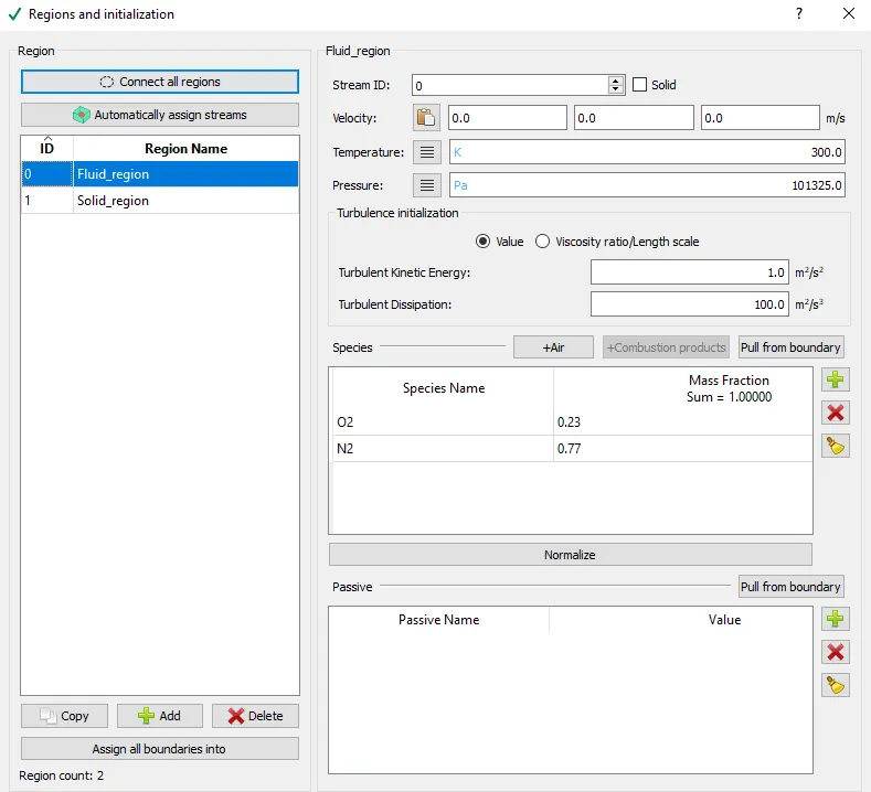
* Before setting up the boundary condition initial conditions are set. Here two regions need to be set one for fluid and other for solid. Fluid region is named as 'Fluid_region' a temperature of 300 K is set along with a pressure of 101325 Pa also the fluid species O2 and N2 needs to be added, the stream id is set to zero (0). Solid region is named as Solid_region and stream id is set as 1 and the box with solid name needs to be checked. Solid species is set as alumininum. A snip of the same is shown below,
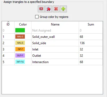
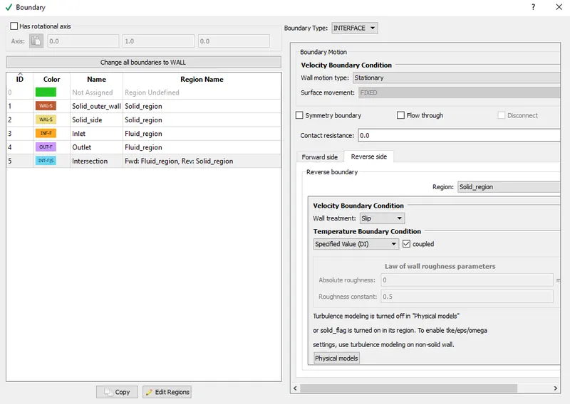
* Since the regions are initialised now the boundary conditions can be set (B.C). Different boundary's of the geometry are flagged as inlet, outlet, intersection and solid side. Below is the snip of the boundary flagging wndow along with the boundary id's.
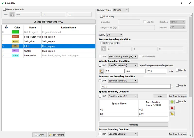
-- For inlet: Boundary type is set as inflow, dirchlet B.C is applied under which inlet velocity is given as input. Inlet velocity is calculated from the input provided in the challenge page,
Reynolds number, Re = 7000 is provided,
We have `R_e = (U*D)/nu`
where, `U -` Inlet velocity (m/s).
`D -` Characteristic length (m).
`nu -` Kinematic viscosity (m^2/s)
since the working fluid is air which enters the inlet through a temperature of 300 K, so kinematic viscosity of air at 300 K is noted
Kinematic viscosity of air at 300K = 1.5757e-05 m^2/s
Characteristic length is nothing but the inlet diameter = 0.015 m
`U = (7000*1.5757e-05)/0.015 = 7.35 m/s`,
hence the inlet velocity is given as 7.35 m/s also the fluid species O2 and N2 are selected along with its mass fraction
-- For outlet: Boundary type is set as outflow, dirchlet B.C is applied under which the value of pressure is set as 101325 Pa, species O2 and N2 are also selected along with its mass fraction.
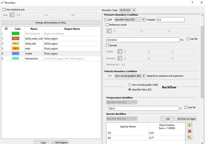
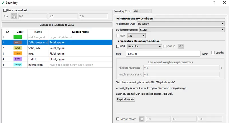
-- For solid_outer_wall : Boundary type is set as wall, wall motion type is set as stationary and surface movement is set as fixed. Slip is also set for the surface movement. Heat flux entering the solid wall is given as temperature boundary condition, heat flux of -10000 w/m^2 is given as input. The -ve sign inicates that the heat is flowing to the solid wall.
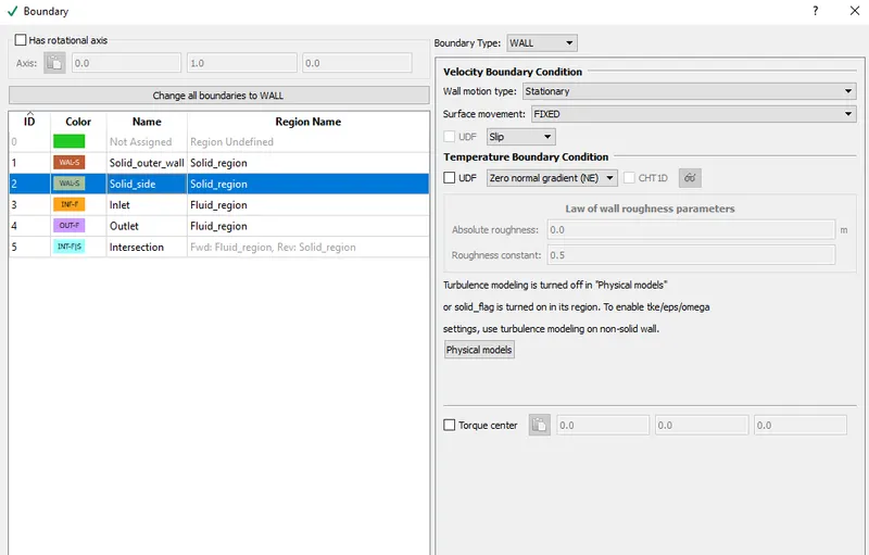
-- For Solid_side: Boundary type is set as wall, wall motion type is set as stationary and surface movement is set as fixed along with slip.Temperature boundary condition is set as zero normal gradient.
-- For intersection: Boundary type is set as interface. Under intersection there are two divisions, they are Forward side and reverse side. Forward side is actually that side where the fluid is flowing and the normals will be pointing in that direction. Velocity boundary condition and temperature boundary condition is set to law of wall.
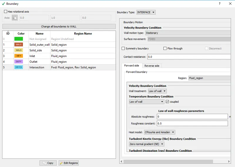
Next comes the reverse side which is the solid region, where the velocity boundary condition is set as slip and temperature boundary condition applied is specified value.
* Once the B.C are set the turbulence model is set to RNG K-ε, also in the physical model local control supercycling is checked. Befor proceeding with setting supercycle local control it is much better to understand what supercycling is and how it is used by converge studio for CHT analysis.
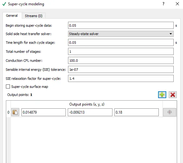
Since the simulation is transient first transient solver solves the navier stokes equation on the fluid region and energy equation on the solid region. After a particular time the average temperature and heat transfer coefficient at the walls are computed and a steady state simulation is run on the solid side, when steady state simulation is run on the solid side the fluid size is freezed, meaning no flow equations are solve on the fluid side. The average wall temperature and heat transfer coefficients are given as B.C for solid side steady state solver.
* The storing of super cycle data is set to start store after 0.05 sec. Solid side solver is set as steady state solver, time length for each cycle stage is set at 0.05 sec also the conduction CFL number is set at 100. A co-ordinate point is also given as input, this point is actually an average taken between 2 vertices of a triangle at the outlet. A snip of the super cycling local contol is shown below,
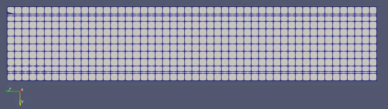
* Grid size is set at 0.004 m initially, grid dependence test is carried further by refining the grid size.
* Also y+ is added in post.in file.
Simulations:
* Grid dependence test is carried out for grid size of 0.004, 0.003 and 0.002 m.
1. For grid size = 0.004 m
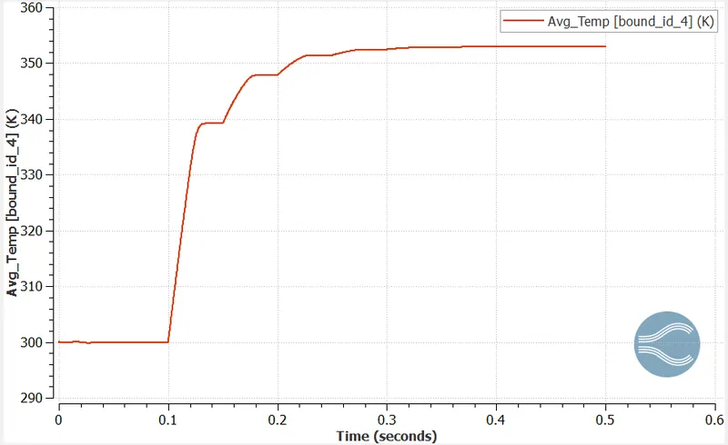
* Temperature profile at outlet:
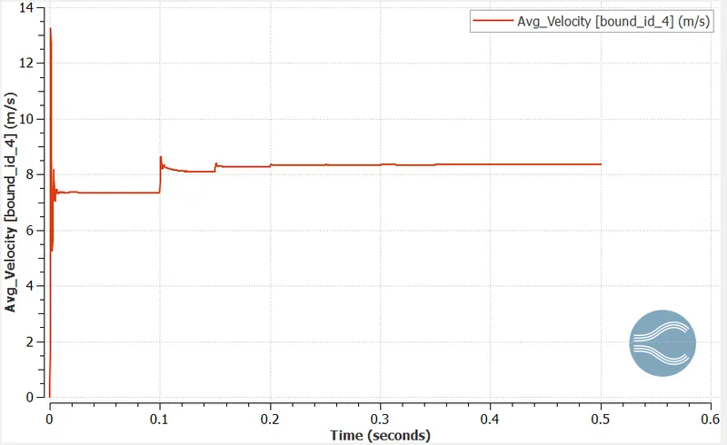
* Velocity profile at outlet:
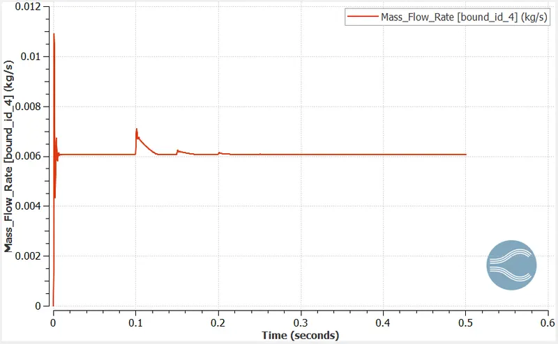
* Mass flow rate at outlet:
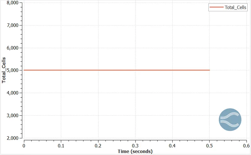
* Cell count plot:
* Generated mesh profile:
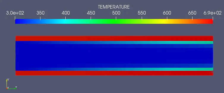
* Temperature contour:
* Temperature contour animation: https://youtu.be/jThYfXd5lzE
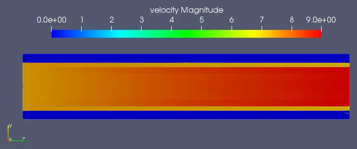
* Velocity contour:
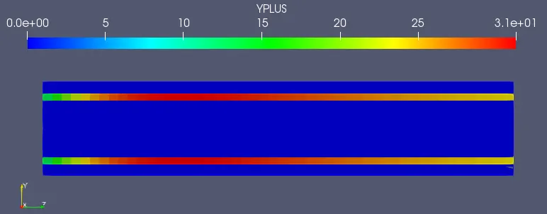
* Y plus contour:
2. For grid size = 0.003 m
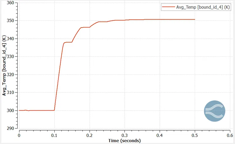
* Temperature profile at outlet:
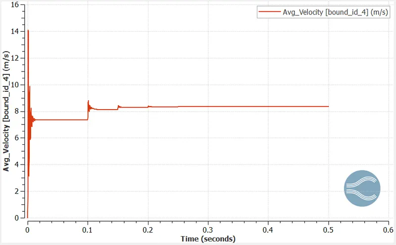
* Velocity profile at outlet:
* Mass flow rate at outlet:
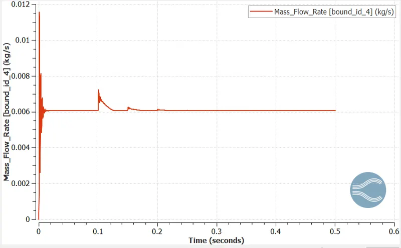
* Cell count plot:
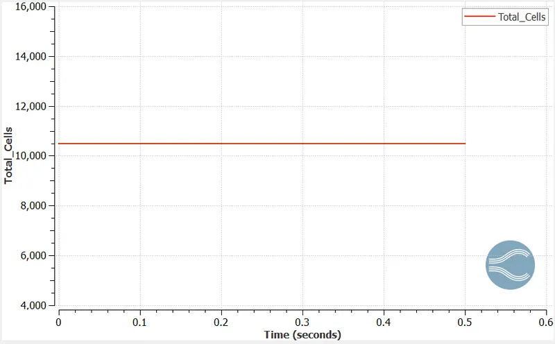
* Generated mesh profile:
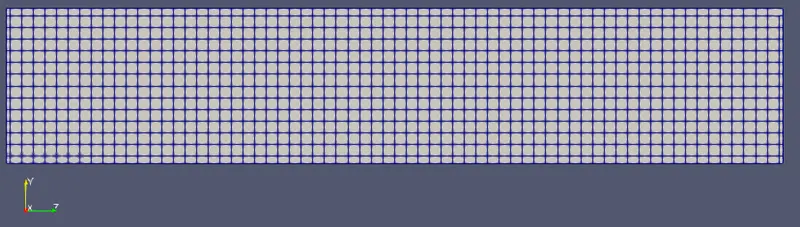
* Temperature contour:
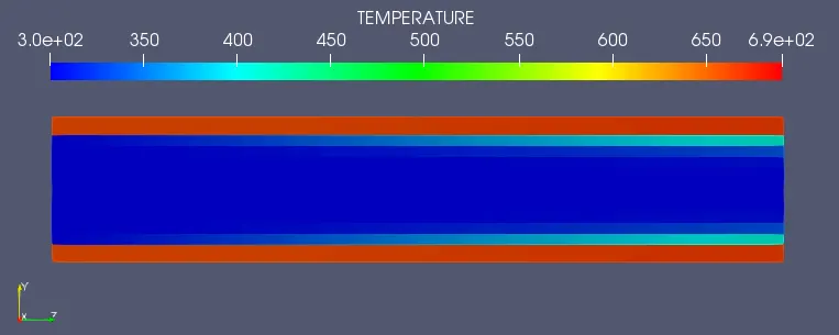
* Temperature contour animation: https://youtu.be/xdUPj8HcRcI
* Velocity contour:
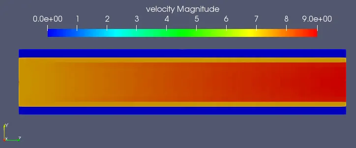
* Y plus contour:
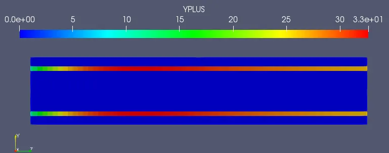
3. For grid size = 0.002 m
* Temperature profile at outlet:
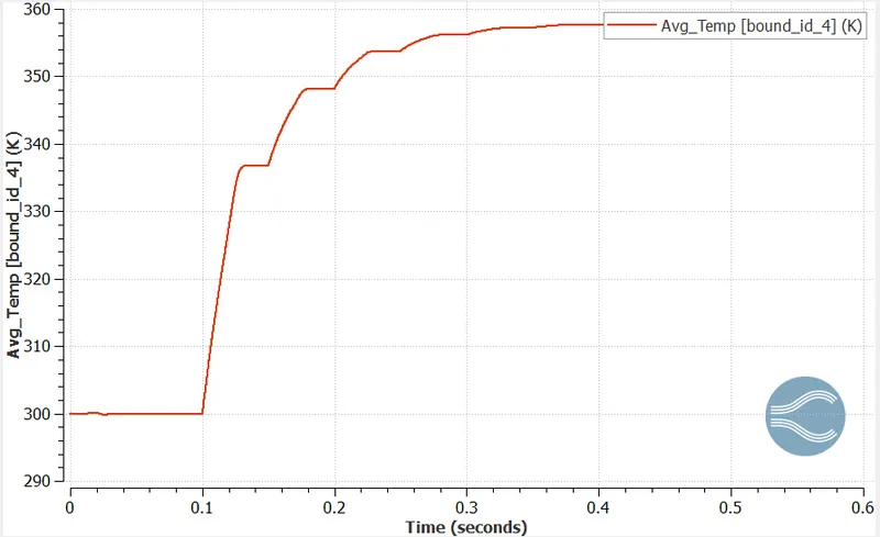
* Velocity profile at outlet:
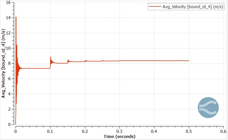
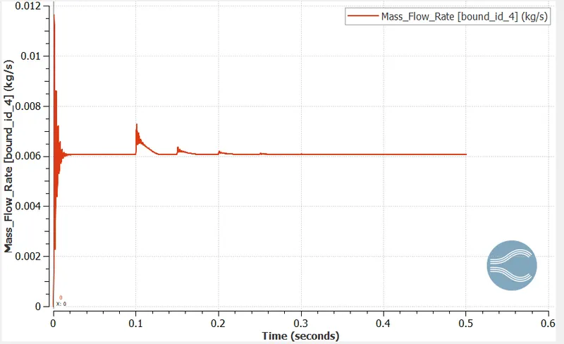
* Mass flow rate at outlet:
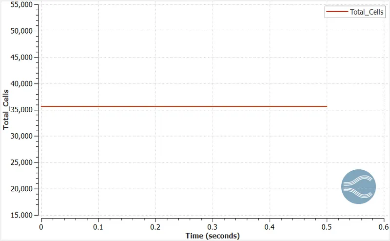
* Cell count plot:
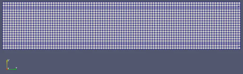
* Generated mesh profile:
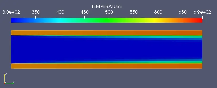
* Temperature contour:
* Temperature contour animation: https://youtu.be/qb5UtK3dp6Y
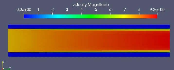
* Velocity contour:
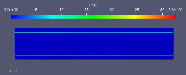
* Y plus contour:
* For base grid size of 0.004 m the super cycle stage interval is set at 0.03, 0.02 and 0.01 sec and the simulation time is noted.
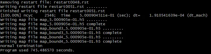
1. Super cycle stage interval = 0.03 sec:
* Above while grid dependence test is carried what ever the result is obtained same is obtained, so those are not repeated hence only the simulation time is shown
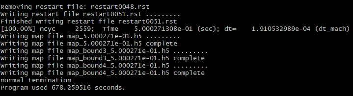
2. Super cycle stage interval = 0.02 sec:
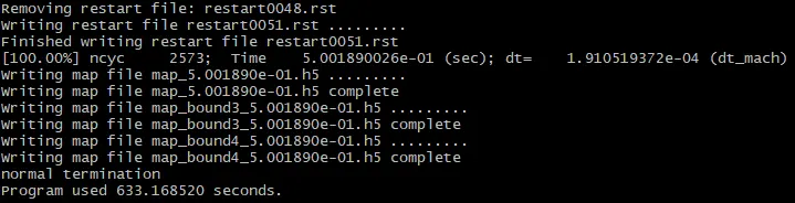
3. Super cycle stage interval = 0.01 sec:
CONCLUSION
* As far as grid dependence test is concerned for all the 3 grid sizes at which simualtions are run the final temperature of fluid at outlet has converged around 360 K
* If velocity and mass flow rate at the outlet is observed it has converged at 8.5 m/s and 0.006 kg/s irrespective of the grid size hence we can define the simulations carried is a grid independence test
* As far as y+ is concerned at grid size of 0.002 m the y+ is between 5 and 30 i.e, the y+ is in the buffer layer, which is not good. For other 2 grid sizes the y+ is much more than 30 which is the log layer. Hence we can conclude that too much refinement beyond 0.003 m is not good.
* As far as the super cycle stage is concerned it is observed that, as we increase the super cycle stage interval the simulation time is also increasing.