Exhaust Port Challenge
# AIM:
* To define what is conjugate heat transfer (CHT) analysis and its purpose.
* To do CHT analysis on exhaust manifold of a inline 4 cylinder engine.
* To choose a right turbulence model and calculate inflation layer thickness using appropriate y+.
* To calculate wall heat transfer coefficient and surface heat transfer coefficient.
# Conjugate heat transfer analysis:
It is heat transfer that takes place between 2 physical bodies, usually between a solid and a fluid. There are many applications in day to day life where we can see a fluid with certain temperature flowing between 2 solid walls and hence heat transfer taking place from fluid to the solid. A good example is engine exhaust where in hot combustion gases transfer heat to the solid exhaust manifold and exhaust manifold inturn transfers heat to the surrounding air. Heat transfer from hot gases to solid exhaust manifold happens through forced convection beacuse combustion gases will be flowing with a certain velocity, through the thickness of the exhaust manifold heat transfer happens by conduction and again from solid surface to surrounding air via natural convection. All heat exchangers fall under same category.
Purpose of CHT is that it can accuratley determine the heat transfer by solving both conduction in solid and forced or natural convection in fluid simultaneously. CHT has an advantage that it can calculate heat transfer which is non uniform which cannot be calculated empirically.
# CHT analysis on exhaust manifold:
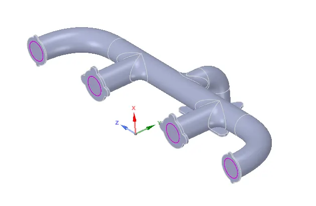
Exhaust manifold of inline 4 cylinder engine is used. In spaceclaim fluid volume is extracted and both solid volume and fluid volume are combined into final geometry. Since this involves 2 physical bodies in contact it is must that we enable share topology option so that information transfer takes place between the 2 bodies. To achieve this in the workbench option there is a tool called share by using it we can make the topology of the final geometry get shared.
Final geometry looks as follow:
* Meshing and Simulations:
Meshing is the important part because it is in this step we decide the type of mesh that we will be using so that we can calculate wall heat transfer coefficient and surface heat transfer coefficients accuratley.
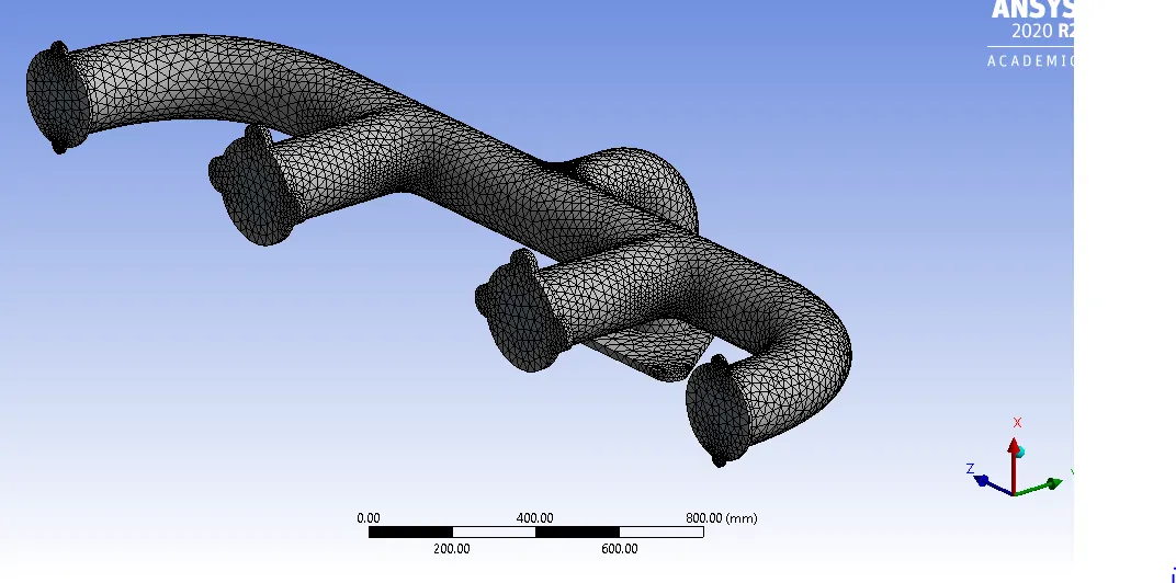
It starts with naming the inlets, outlet, outer_wall_convection and inflation_layers. circular projections on the inlets and triangular base on the outlet is not named, they are treated as adiabiatic. Once naming is done base line mesh is generated. After applying baseline mesh geometry looks as follow:
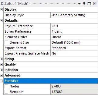
A snip of the number of cells in the baseline mesh is given below,
* Solver setup:
Steady state simulations are carried, using a pressure based solver. Energy equation is selected since we are interested in knowing the temperature distribution on the outer solid wall. since k-omega model is better in capturing wall phenomena also wall heat transfer coefficient is to be calculated k-omega turbulence model is used.
Fluid is used as air, on the solid side aluminium is used. After that boundary conditions are set to the named selections. Inlet is set as velocity boundary and hence inlet velocity is set as 5 m/s and inlet temperature is set as 700 K. Outlet is set as pressure boundary condition. So in outlet atmospheric gauge pressure is set which is nothing but 0 Pa. Outer_wall convection is set as covective boundary condition and hence we have to provide convective heat transfer coefficient h (W/m^2.K) as input. h is provided as 20 W/m^2 K.
To view the results after the calculations are complete, temperature contour is added also a solution animation of the same is created. Simulations are run for 150 iterations.
After running the simulations for base line mesh, coefficient of wall heat transfer coefficient and surface heat transfer coefficient are calculated.
* Temperature distribution:
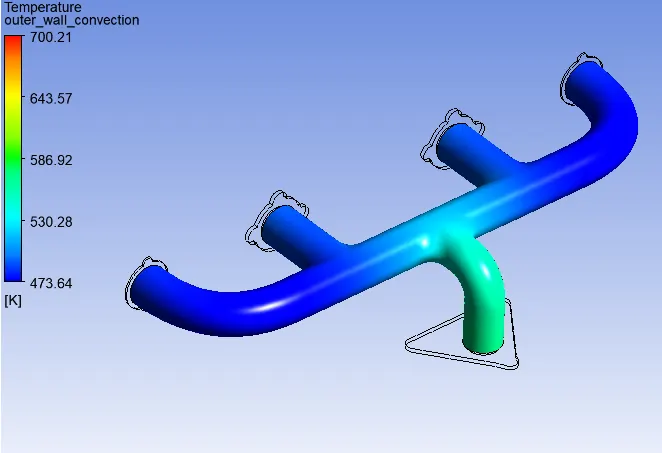
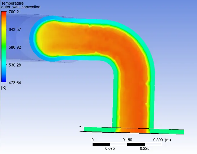
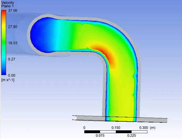
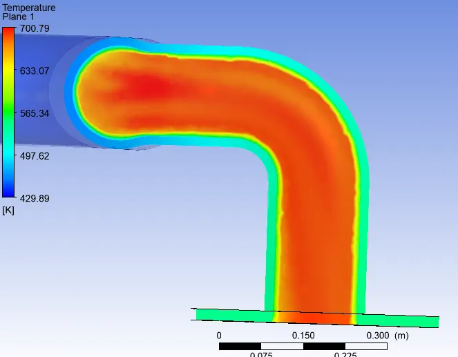
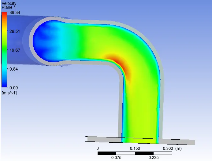
From the above contour plot it is observed that temperature is more near the outlet rather than near inlet, reason for this is forced convection. As velocity increase convection increases, so near outlet where exhaust gases from all the ports meet velocity will be higher and hence more temperature is observed near outlet. This can be further established by observing the temperature contour and velocity contour on a slice plane inserted at the outlet.
* Temperature contour:
* Velocity contour:
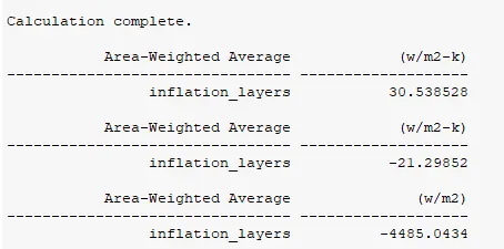
also Wall heat transfer coefficient, surface heat transfer coefficient and surface heat flux are also calculated
Wall heat transfer coefficient = 30.538528 W/m^2-k.
Surface heat transfer coefficient = -21.2852 W/m^2-k.
Surface heat flux = -4485.0434 W/m^2.
a snip of the same is attached below,
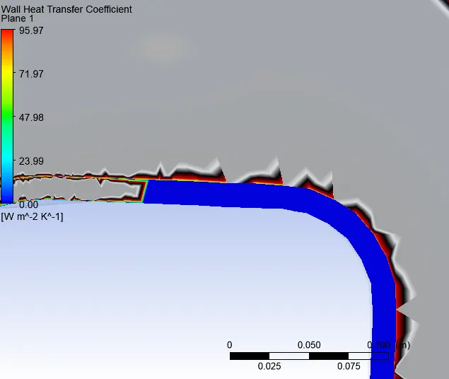
* Wall heat transfer coefficient:
* Refined Mesh:
Since all the above results were obtained for base line mesh, it is necsessary that we refine the mesh and observe the result and check how it is different from the base line mesh. Mesh refinement is achieved by using local controls. One of the important aspect of mesh refinement is addition of inflation layers. Since we are using k-omega tyrbulence model it is essential that we keep our y+ value below 5.
we have y-plus given as, `y+ = (rho*U_(tau)*y)/mu`
where, `rho` - Density (kg/m^3).
`U_(tau)`- Velocity (m/s).
`y` - First layer thickness (m).
`mu` - dynamic viscosity (Kg/m-s).
from the above equation we have , `y = ((y+)*mu)/(rho*U_(tau))`
also we have , `U_(tau) = sqrt(tau_(w)/rho)`
`tau_(w) = 1/2*C_(f)*rho*U^2`
where, `C_(f)` - Skin friction coefficient.
`C_(f) = 0.058*Re^-0.2`
So it is obvious from the above formula's that it all starts with calculation of Reynolds number.
Reynolds number, `Re = (U*D)/nu`
`U` - Velocity (m/s).
`D` - Characteristic length (m). (here it is the dia. of the inlets)
`nu` - Kinematic viscosity (m^2/s).
We have inlet velocity of u = 5 m/s. since air is the fluid considered for air we have,
`nu = 1.4607*10^-5`
`D = 0.17 m`
therefore, `Re = (5*0.17)/(1.4607*10^-5) = 58.19*10^3`
since this is an internal flow Re > 2300 can be considered as turbulent flow.
we have, `C_(f) = 0.058*(58.19*10^3)^-0.2` = 6.35 * 10^-3
`tau_(w) = 1/2*6.35*10^-3*1.225*5^2` = 0.097 N/m^2.
`U_(tau) = sqrt(0.097/1.225) = 0.281 m/s`
so here y+ = 1.25 is taken for calculating the first layer thickness, y = (1.25*1.7894*10^-5)/(1.225*0.281) = 0.06497 * 10^-3 m = 0.06497 mm
hence we have first layer thickness, y = 0.06497 mm, so for 5 layers with growth rate of 1.2 total thickness = 0.06497 * 1.2^5 = 0.161 mm.
so this total thickness is inserted while adding inflation layers. Inflation layers are added on the surface of fluid volume, it looks as follow
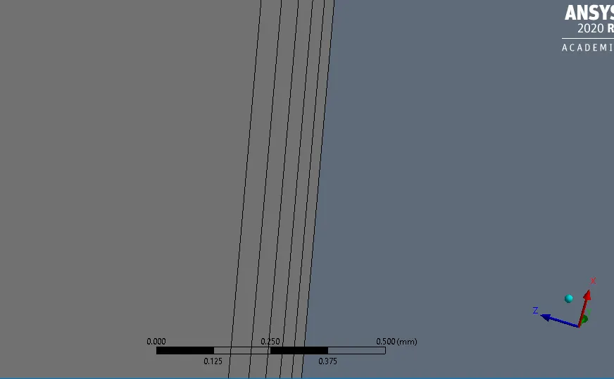
*Plot of Y+:
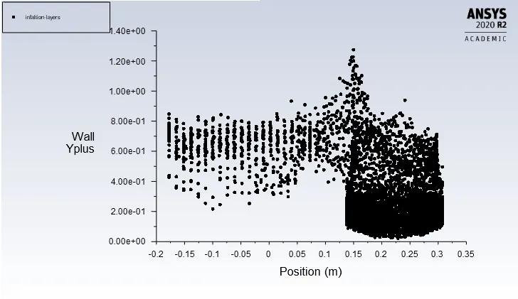
from the above y+ plot it is clear that all the points on the surface on which inflation layers are applied are well within the limit.
other than inflation layers edge sizing is added on to the edges at the inlet and outlet, with a total number of 18 divisions. Also body sizing is added on to the fluid volume with an element size = 15 mm. So the refined mesh has more number of cells than baseline mesh. A grab of the cell count for the refined mesh is given below,
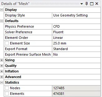
Refined mesh looks as follow,
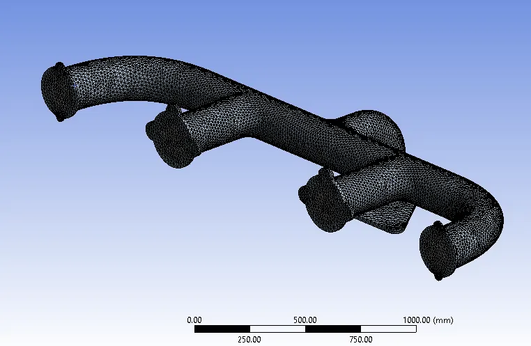
once the mesh is refined solution is ran for 150 iterations and the results are observed.
* Temperature distribution:
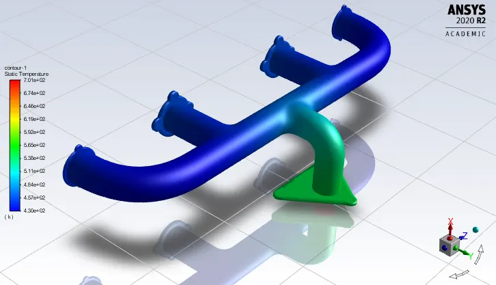
* Temperature contour:
* Velocity contour:
Wall heat transfer coefficient = 22545.4124 W/m^2-k.
Surface heat transfer coefficient = -20.7362 W/m^2-k.
Surface heat flux = -3552.3803 W/m^2.
a snip of the same is attached below,
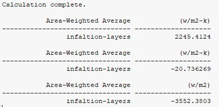
* It is observed that when inflation layers are added the wall heat transfer coefficient have increased drastically, which implies that heat transfer do takes place from fluid volume to solid volume. To know it better it will be good if we go for refinement by adding inflation layers.
* If we compare the value of surface heat transfer coefficient in baseline mesh and above refined mesh it is almost the same or else we can say that the change is not significant and it is grid independent.
* Wall heat transfer coefficient:
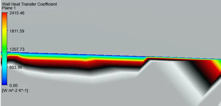
To confirm the result further mesh independent study can be done.
Suppose if we choose a y+ = 2, mesh count will change.
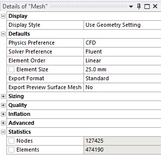
For above cell count, simulations are run for 150 iterations and results are observed.
Wall heat transfer coefficient = 1939.8603 W/m^2-k.
Surface heat transfer coefficient = -20.895141 W/m^2-k.
Surface heat flux = -4043.6337 W/m^2.
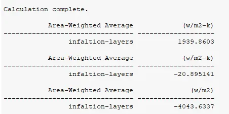
so it can be observed that for y+ = 2 the wall heat transfer coefficient is less compared to that of y+ = 1.25 this is because for y+ = 1.25 first layer is much closer than at y+ = 2. Surface heat transfer coefficient is almost the same.
* Accuracy of the result depend on following points:
1. Accurate modelling of the problem.
2. Geometry should be good enough so that it does not disturbs the flow physics.
3. The residuals should fall below the threshold value for a given goemetric model.
4. Selection of solution model and methodology.
5. Materials selection is of due importance, if same materials are used which are used in practical applications then it will be easier to verify the results.