Week 5: Prandtl Meyer Shock problem
AIM
* To explain what is a shock wave.
* To explain different types of boundary conditions used in shock wave problems.
* To explain effect of SGS on cell count and shock.
INTRODUCTION
Shock waves are type of propagating disturbances that move faster than the local speed of sound in the medium. Like an ordinary wave shock waves carry energy and it can propagate through medium, but is characterized by an abrupt nearly discontinous change in pressure, temperature and density of the medium. Shock waves are formed as a pressure front moves at supersonic speed and pushes on the surrounding air. At the point where this occurs there comes a region where the sound waves travelling against flow cannot move further upstream and pressure progressivley builds in that region, a high pressure shock wave rapidly forms.
Shock waves are not conventional sound waves. A shock wave takes the form of a very sharp change in gas propeties. A shock wave is one of different ways in which a gas under supersonic flow can be compressed.
Since this is a simulation run to observe prandtl meyer shock waves, it becomes relevant to explain little bit about prandtl meyer shock waves. When a supersonic flow encounters a conver corner it forms an expansion fan which consists of infinite number of expansion waves centered at corner these expansion waves are called as prandtl meyer expansion waves.
Boundary condition: For shock wave encountered CFD problems usually dirchlet B.C is used where the inlet velocity of the gas is mentioned. At outlet also same dirchlet boundary condition is used.
SIMULATIONS
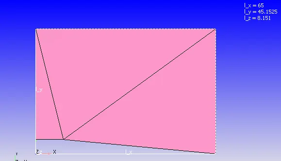
Geometry: A simple geometry with a convex corner is used for simulation. The geometry along with the dimensions is shown below,
Solver setup:
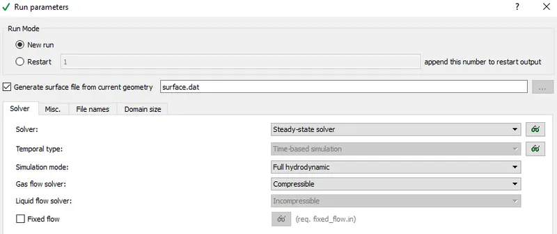
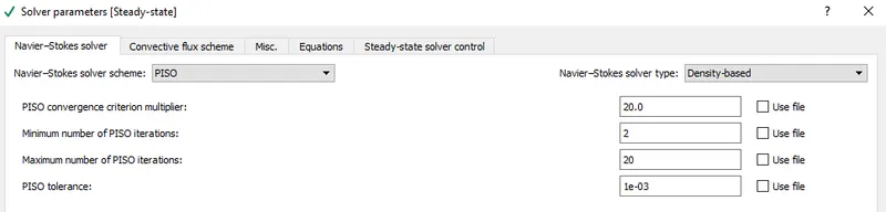
A 2D simulation is carried out for flow of gas through the above shown geometry. A steady state simulation is run using a density based solver. Reason for using a density based solver is because of the compressible nature of the gas flowing at supersonic speeds. A snip of the same is shown below,
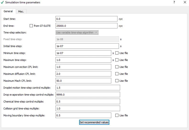
* Since a steady state simulation is carried out start time is set at 0 cycle and end time is set at 25000 cycles. Also initial time and minimum time is set at 1e-7 cycles and max. time is set at 1 cycles.
* 5 boundary's were assigned to the geometry which includes inlet, outlet, front, back and Top-bottom. At inlet dirchlet B.C is used and inlet velocity of 680 m/s and inlet temperature of 286.1 K is given also air with its constituents as O2 and N2 was set.
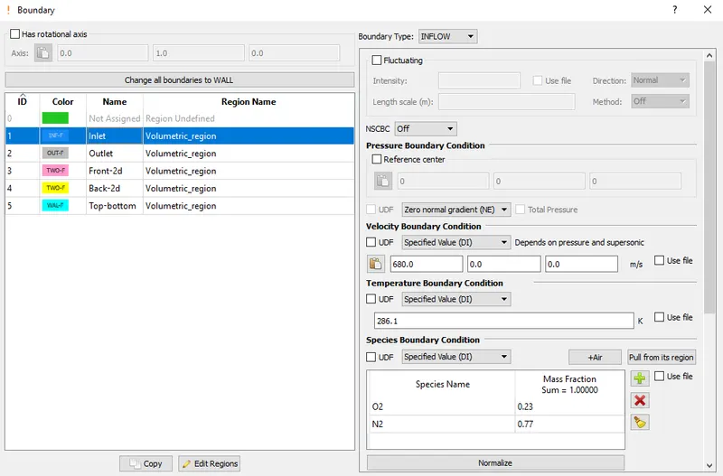
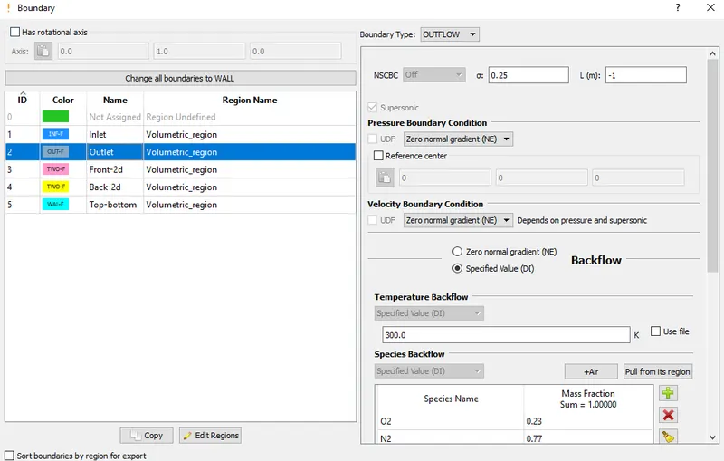
* At outlet same dirchlet boundary condition is used, since the value of outlet pressure and velocity were not known it was set as zero normal gradient. Same as inlet at outlet also air with its constituents as O2 and N2 was set.
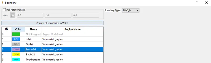
* Since 2D simulation is carried out, for front and back faces 2-D boundary condition is applied.
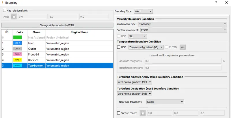
* For Top-bottom wall slip B.C is applied and since temperature at the walls were unknown it is set as zero normal gradient.
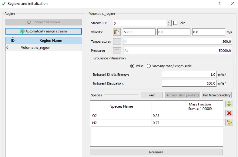
* The fluid domain is initialised with values specified for temperature, velocity and pressure. Initialised fluid volume is named as volumetric region, air with its constituents O2 and N2 is also set here. A snip of the same is provided below,
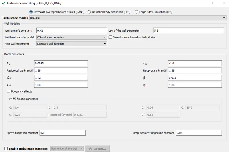
* As far as turbulence model is concerned, RNG K-ε is set.
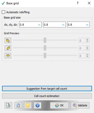
* A grid size of 0.8 m is used for the given dimensions of the geometry. To accuratley capture the shock waves Adaptive-mesh refinement (AMR) is used. AMR local controls can be activated using the options under the Grid controls tab. A snip of the base grid size used as well as the local controls under AMR is shown below,
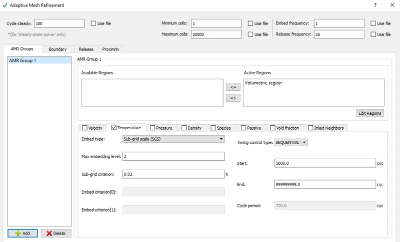
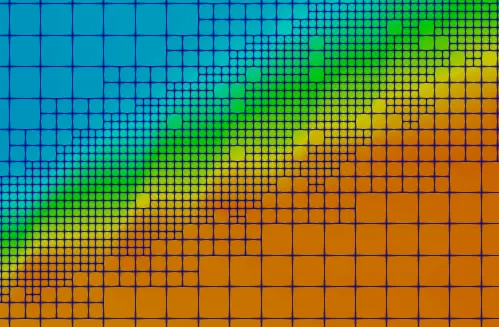
Under AMR local controls the maximum cells is set as 200000, all the defined fluid volume's can be seen under the available region, required region is selected and shift under active region's. There are different factors based on which the cell refinement takes place. As seen from the above velocity, tempeature, density etc. can be used as the parameters to determine the mesh refinement. In this simulation temperature is used as parameter to determine the refinement.
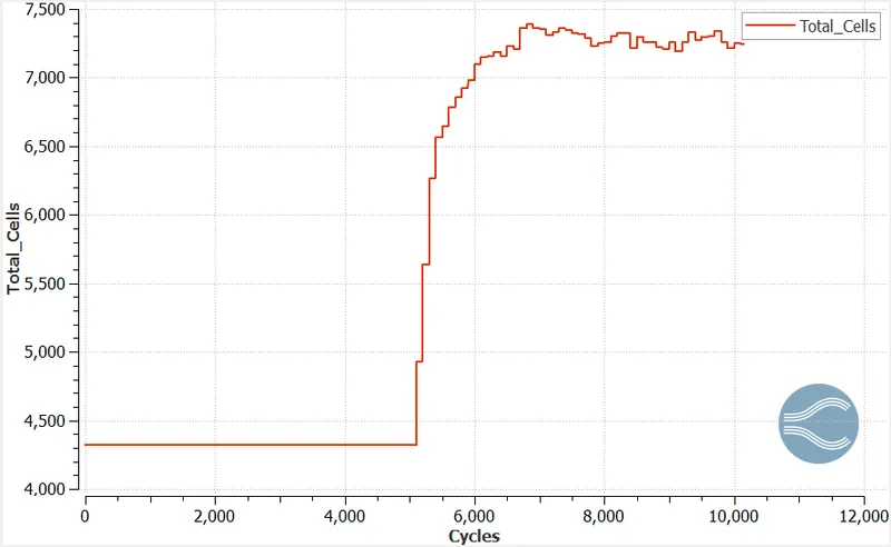
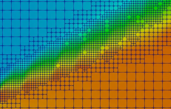
Under the temperature tab the max embedding level is set as 2. Also the embed type is set as Sub grid scale, Sub grid criterion is set as 0.02 K i.e as the temperature difference between the grid becomes 0.02 K refinement takes place. Refinement start time and end time can also be set using the local controls under the temerature tab. Start cycle is set as 5000 and end cycle is set as 999999999.0. All the other local controls under the AMR tab is left as it is.
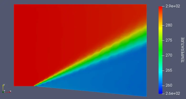
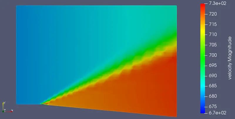
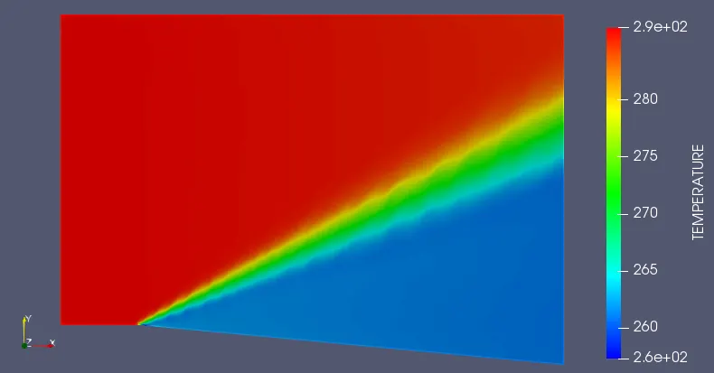
* Simulation is mainly run to observe the effect of SGS on cell count and shock waves. First the simulation is run for a value of SGS = 0.05 K and it is refined further as 0.03 and 0.02 K and the observations are noted.
1. For SGS = 0.05 K
* Temperature contour:
* Temperature contour animation: https://youtu.be/okFuTqKZSBY
* Velocity contour:
* AMR:
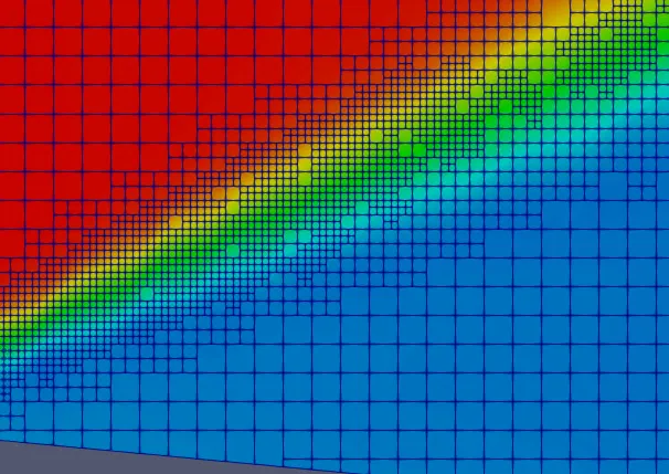
* Cell count plot:
2. For SGS = 0.03 K
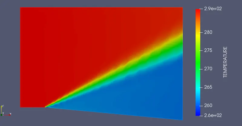
* Temperature contour:
* Temperature contour animation: https://youtu.be/vsUBK00x-5I
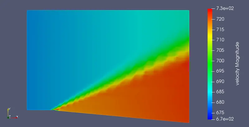
* Velocity contour:
* AMR:
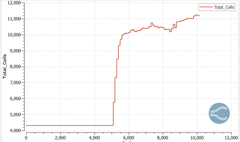
* Cell count plot:
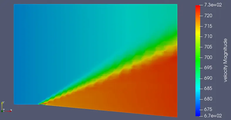
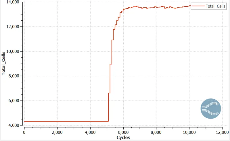
3. For SGS = 0.02 K
* Temperature contour:
* Temperature contour animation: https://youtu.be/AjBeFbW6fL4
* Velocity contour:
* AMR:
* Cell count plot:
CONCLUSION
* As the SGS value is refined, the cell count has increased. The increment in the cell count started around 5000 cycles, which is the start time set for AMR using the local controls.
* As the SGS value is refined the shock wave has become sharp, i.e the shocks are not much dispersed. This can be clearly observed in the velocity contour.