Week 5 - Literature review: ODE Stability
AIM
* To understand stability of ODE and its significance in engineering simulations.
INTRODUCTION
In the last challenge the rate of production of each species in the given reaction mechanism is computed the resulting formulation obtained is nothing but a matrix of ODE's as shown below.
`[[omega_1],[omega_2],[omega_3],[omega_4],[omega_5],[omega_6],[omega_7]] = [[d/dt[X_1]],[d/dt[X_2]],[d/dt[X_3]],[d/dt[X_4]],[d/dt[X_5]],[d/dt[X_6]],[d/dt[X_7]]]`
above ODE's need to be solved in a computer and hence it becomes neccessary that we understand how the given or derived ODE's can be descritized and what effects the stability of such ODE's.
* When does a ODE become unstable ?
To understand this let us consider a ode given as `(dY)/dx = -lamda*Y`
the ode can be discretized as, `(Y_(n+1) - Y_n)/(Deltax) = -lamda*Y_n`
`Y_(n+1) = Y_n - lamda*Y_n*Deltax` , this type of dicretization is called explicit form. The discretizedform can be further simplified as,
`Y_(n+1) = Y_(n)*(1-lamda*Deltax)`
For the soution to be stable the condition is that as the value of independent variable increases the solution should decrease or should be fixed or should be at equilibrium.
It is called explicit form because to compute the value of Y at a point (`Y_n`) the values of Y at previous points (`Y_(n-1)`) is used. Stability of ode discretized by explicit form is given as
`abs(1-Deltax*lamda) lt 1` simplifying further we have
`2/lamda gt Deltax gt 0`
from the above expression it is clear that value of both `lamda, Deltax`determines the stability of ode. To understand this better let us consider a ode as given below,
`(dY)/dt = -1000*Y - exp(-t)`
for the above given ode the RHS can be considered as a function of t, `f(t)`
discretizing the above ode explicity we have, `(Y_(n+1) - Y_n)/(Deltax) = f(t)`
`Y_(n+1) = Y_n + Deltax*f(t)`
To solve a program is written using python as shown below,
"""
Understanding ODE stability
"""
import math

import matplotlib.pyplot as plt

def f(t,y):

	c = -1000*y - math.exp(-t)

	return c

t_start = 0

t_end = 0.1

No_of_points = 500

dt = (t_end - t_start)/(No_of_points-1)

t = 0

y_old = 0

y_new = []

for i in range(0,No_of_points+1):

	y_new.append(y_old + f(t,y_old)*dt)

	y_old = y_new[i]

	t = t + dt


plt.plot(y_new)
plt.show()
Executing the above program gives the below plot of Y,
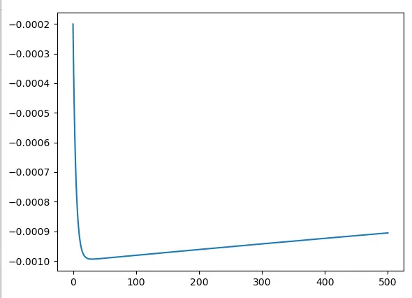
we have `Deltat = (0.1-0)/(500-1) = 0.0002`
we have `lamda = 1000`hence `2/lamda = 0.002`, hence `2/lamda gt Deltat gt 0` this stability criterion is satisfied and hence the solution is stable`
* For the same ode if we decrease the number of points (grid) to 50 we have,
`Deltat = (0.1-0)/(50-1) = 0.002` also we have `2/lamda = 0.002`, under this condition the stability criterion is not satisfied and hence the solution should be unstable and this is evident from the plot of y obtained, as given below.
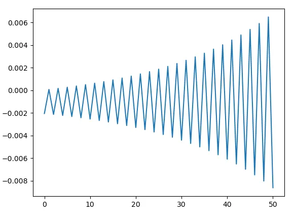
* Hence we can conclude that ode discretized by explicit form becomes unstable accordingly with the grid size. But the same can be compensated by changing the value of `lamda`.
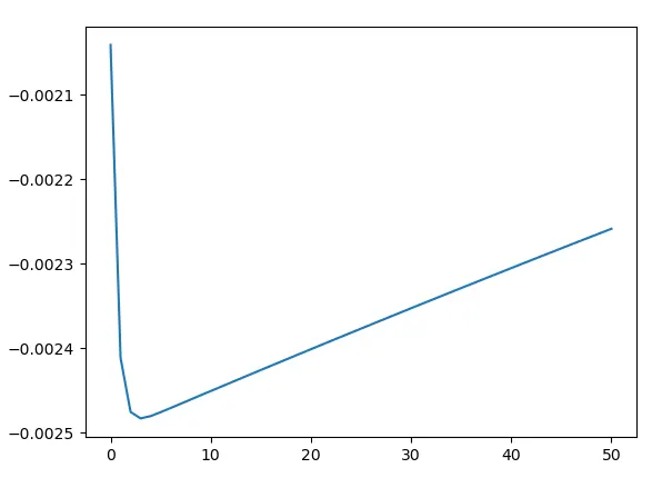
In the above case for a grid size of 50 the stability criterion is not satisfied. Suppose if we reduce the value of `lamda`to 400,
we have `Delta t = (0.1-0)/(50-1) = 0.002`
and `2/lamda = 2/400 = 0.005` , and hence the stability criterion `2/lamda gt Deltat gt 0` is satisfied, and this is evident from the plot of Y as shown below`
* Another way of discretizing the ode is implicitly. Consider the same ode, `(dY)/dt = -lamda*Y` , discretizing implicitly we have,
`(Y_(n) - Y_(n-1))/(Deltax) = -lamda*Y_(n)`
`Y_n-Y_(n-1) = -lamda*Y_n*Deltax`
`Y_n+lamda*Y_n*Deltax = Y_(n-1)`
`Y_n*(1+lamda*Deltax) = Y_(n-1)`
`Y_n = Y_(n-1)/(1+lamda*Deltax)` , Stability of this ode is given as `1/(1+lamda*Deltax) < 1`and this criteria is met for all `Deltax gt 0` and hence we can say that this ode is absolutley stable.
If we consider the example case, `(dY)/dt = -1000*Y - exp(-t)`
`(Y_n - Y_(n-1))/(Deltat) = -1000*Y_n - exp(-t)`
`Y_n - Y_(n-1) = (-1000*Y_n - exp(-t))*Deltat`
`Y_n-(-1000*Y_n-exp(-t))*Deltat = Y_n-1`
`Y_n + 1000*Y_n*Deltat + exp(-t)*Deltat = Y_(n-1)`
`Y_n(1+1000*Y_n*Deltat) = Y_(n-1)-exp(-t)*Deltat`
`Y_n = (Y_(n-1)-exp(-t)*Deltat)/(1+1000*Deltat)`
* Above discretized form can be solved by writing a code in python. Both implicit and explicit results are compared in a single code as shown below,
"""
Understanding ODE stability
"""
import matplotlib.pyplot as plt

import math

import numpy as np

def explicit_method(t_total,dt):

	t = np.arange(0,t_total,dt)

	y = np.zeros(len(t))

	for i in range(1,len(t)):

		y[i] = (-1000*y[i-1]-np.exp(-t[i-1]))*dt + y[i-1]


	return [t,y]


def implicit_method(t_total,dt):

	t = np.arange(0,t_total,dt)

	y = np.zeros(len(t))

	for i in range(1,len(t)):

		y[i] = (y[i-1]-np.exp(-t[i-1])*dt)/(1+1000*dt)


	return [t,y]

t_total = 0.1

dt = 1.9e-04

t,y_explicit = explicit_method(t_total,dt)

t,y_implicit = implicit_method(t_total,dt)

plt.plot(y_explicit)
plt.plot(y_implicit)
plt.legend(['explicit','implicit'])
plt.show()
* Executing the above we get the below plot,
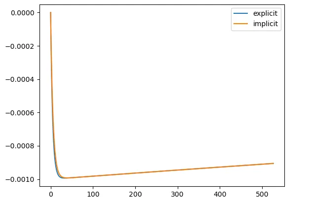
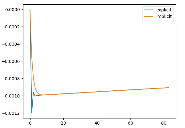
which implies that both implict and explicit methods are stable for dt = 1.9e-04, now if dt is changed to 1.2e-03 and the above code is executed we get the solution plot as,
further changing the value of dt = 1.9e-03,
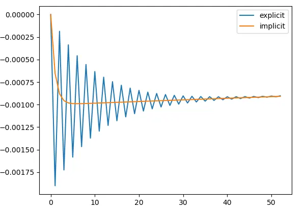
* It shows that for any value of `Deltat gt 0` the implicit formulation is stable since the stability criteria of `1/(1+lamda*Deltax) lt 1` is always satisfied, but the explicit formulation blows up as the stability criteria of `2/lamda gt Deltax gt 0` is not satisfied
* How does stability affect engineering simulation?
As far as engineering simulations are concerned stable solutions are relaible, i.e, the solution should reach a equilibrium after certain point. Unstable solutions are characterised by large oscillations or changes in the solution which does not die down or stabilize even after a certain point such solutions are not at all useful in engineering simulations. If the oscillations in the solution die down or disappears as we progress then such a solution is reliable.
* Can stability condition can be derived for all type of problems?
Stability conditions can only be derived for linear ode's. For non-linear ode's it is possible by defining a jacobian matrix. Jacobian matrix is nothing but a matrix of first order derivatives of all the functions w.r.t all the independent variables. Eigen value of the jacobian matrix is computed, if all the eigen values are negative then the ode is said to be stable if one of the eigen value is positive then the solution becomes unstable.